Properties of the Transmon
Ref: DOI:10.48550/arXiv.2203.04164
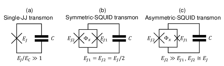
As mentioned previously, Josephson junctions exhibit inductive properties, and the Transmon is a variant of an LC circuit where the inductance is replaced by a Josephson junction. This section directly discusses the Tunable Transmon, where a SQUID is used as the inductance. In practice, due to material inhomogeneity, different Transmons may have different properties. However, by using a Tunable Transmon, the qubit properties can be made consistent by fine-tuning the magnetic flux \(\Phi_B\). Additionally, as we discussed earlier when quantizing the LC circuit, \([ \Phi, Q ] = i\hbar\) are conjugate variables. Using the derivation for the SQUID, we can naturally relate the magnetic flux \(\Phi\) to the phase difference \(\Delta\theta\), i.e.: \[ \Phi \equiv \frac{\Delta\theta_1}{\pi} \Phi_0 - \Phi_B. \]
Now, we write down the Hamiltonian: \[ \mathcal{H} = \frac{Q^2}{2C} + \frac{\Phi_\#^2}{2L} = \frac{Q^2}{2C} + \frac{(I_0 \pi)}{2\Phi_0} \cos\left(\frac{\Phi_B}{\Phi_0} \pi\right) \Phi^2 - \frac{I_0}{24} \left(\frac{\pi}{\Phi_0}\right)^3 \cos\left(\frac{\Phi_B}{\Phi_0} \pi\right) \Phi^4 + \cdots \] \[ = \frac{Q^2}{2C} + \frac{\Phi^2}{2L} - \frac{1}{24L} \left(\frac{\pi}{\Phi_0}\right)^2 \Phi^4 + \cdots \] where: \[ L = \left(\frac{I_0 \pi}{\Phi_0} \cos\left(\frac{\Phi_B}{\Phi_0} \pi\right)\right)^{-1}. \]
Next, we discuss how the nonlinearity affects the energy levels. From earlier, we selected new variables \( a \), \( a^\dagger \): \[ a = \sqrt{\frac{1}{2\hbar} \sqrt{ \frac{L}{C}}} \left(\sqrt{\frac{C}{L}} \Phi + iQ\right), \quad a^\dagger = \sqrt{\frac{1}{2\hbar} \sqrt{ \frac{L}{C}}} \left(\sqrt{\frac{C}{L}} \Phi - iQ\right). \] Conversely: \[ \Phi = \sqrt{\frac{\hbar}{2 }\sqrt{ \frac{L}{C}}} (a^\dagger + a), \quad Q = i\sqrt{\frac{\hbar}{2} \sqrt{ \frac{C}{L}}} (a^\dagger - a). \]
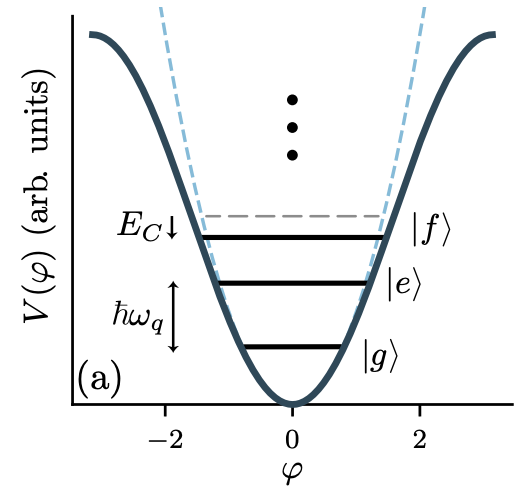
Expanding the Hamiltonian: \[ \mathcal{H} = \frac{\hbar}{\sqrt{LC}} \left[a^\dagger a + \frac{1}{2}\right] - \frac{1}{24L} \left(\frac{\pi}{\Phi_0}\right)^2 \left[i \sqrt{\frac{\hbar}{2\sqrt{L/C}}} (a^\dagger + a)\right]^4. \] Simplifying: \[ \mathcal{H} = \frac{\hbar}{\sqrt{LC}} \left[a^\dagger a + \frac{1}{2}\right] - \frac{\hbar^2}{96C} \left(\frac{\pi}{\Phi_0}\right)^2 (a^\dagger + a)^4. \] This expression contains both linear and nonlinear terms, where the linear terms describe the energy levels of a quantum harmonic oscillator, and the nonlinear terms arise from the Josephson junction's correction to the energy levels.
Using perturbation theory, when \( \mathcal{H} = H_0 + \Delta H \), and \( |E_0^m\rangle \to |E^m\rangle \), \( E_0^m \to E^m = E_0^m + \delta E^m \), we know the energy correction \( \delta E^m \) to the energy level \( E_0^m \) is:
\[ \delta E^m = \langle E_0^m | \Delta H | E_0^m \rangle = \langle E_0^m | \left[-\frac{\hbar^2}{96C} \left(\frac{\pi}{\Phi_0}\right)^2 (a^\dagger + a)^4\right] | E_0^m \rangle. \]
Expanding this:
\[ \langle E_0^m | (a^\dagger + a)^4 | E_0^m \rangle = \langle E_0^m | (aa + aa^\dagger + a^\dagger a + a^\dagger a^\dagger)^2 | E_0^m \rangle. \]
Expanding further:
\[ \langle E_0^m | aa(aa + aa^\dagger + a^\dagger a + a^\dagger a^\dagger) + aa^\dagger(aa + aa^\dagger + a^\dagger a + a^\dagger a^\dagger) + a^\dagger a(aa + aa^\dagger + a^\dagger a + a^\dagger a^\dagger) + a^\dagger a^\dagger(aa + aa^\dagger + a^\dagger a + a^\dagger a^\dagger) | E_0^m \rangle. \]
Taking the expectation value, we only keep terms where \( a \) and \( a^\dagger \) appear with equal powers, resulting in:
\[ \langle E_0^m | aaa^\dagger a^\dagger + aa^\dagger aa^\dagger + aa^\dagger a^\dagger a + a^\dagger aaa^\dagger + a^\dagger aa^\dagger a + a^\dagger a^\dagger aa | E_0^m \rangle. \]
Simplifying further:
\[ \langle E_0^m | a(a^\dagger a + 1)a^\dagger + aa^\dagger aa^\dagger + (a^\dagger a + 1)a^\dagger a + a^\dagger a(a^\dagger a + 1) + a^\dagger aa^\dagger a + a^\dagger (aa^\dagger - 1)a | E_0^m \rangle. \]
Further simplifying:
\[ \langle E_0^m | aa^\dagger aa^\dagger + aa^\dagger + aa^\dagger aa^\dagger + a^\dagger aa^\dagger a + a^\dagger a + a^\dagger aa^\dagger a + a^\dagger a + a^\dagger aa^\dagger a + a^\dagger aa^\dagger a - a^\dagger a | E_0^m \rangle. \]
After further simplification:
\[ \langle E_0^m | 2aa^\dagger aa^\dagger + aa^\dagger + 4a^\dagger aa^\dagger a + a^\dagger a | E_0^m \rangle. \]
This simplifies to:
\[ \langle E_0^m | 2(a^\dagger a + 1)(a^\dagger a + 1) + (a^\dagger a + 1) + 4a^\dagger aa^\dagger a + a^\dagger a | E_0^m \rangle. \]
Finally, the energy level correction is:
\[ \langle E_0^m | 6a^\dagger aa^\dagger a + 6a^\dagger a + 3 | E_0^m \rangle = 6m^2 + 6m + 3. \]
The energy difference between levels \(m\) and \(m-1\) is:
\[ \Delta E^m_{m-1} = \frac{\hbar}{\sqrt{LC}} - \frac{\hbar^2}{96C} \left(\frac{\pi}{\Phi_0}\right)^2 \left\{6[m^2 - (m-1)^2] + 6\right\}. \]
\[ = \frac{\hbar}{\sqrt{LC}} - \frac{\hbar^2 \pi^2}{96C} \frac{e^2}{\pi^2 \hbar^2} \left[6(2m - 1) + 6\right]. \]
Finally, we get:
\[ \Delta E^m_{m-1} = \frac{\hbar}{\sqrt{LC}} - m\frac{e^2}{8C}. \]
Calculating \( \Delta E^{21} - \Delta E^{10} \):
\[ \Delta E^{21} - \Delta E^{10} = \left(\frac{\hbar}{\sqrt{LC}} - 2\frac{e^2}{8C}\right) - \left(\frac{\hbar}{\sqrt{LC}} - \frac{e^2}{8C}\right). \]
\[ = -\frac{e^2}{8C} \equiv -E_C. \]
\( E_C \) represents the nonlinear effect.
Ref: DOI:10.1103/RevModPhys.93.025005
Originally written in Chinese by the author, these articles are translated into English to invite cross-language resonance.
 Peir-Ru Wang