Qubit Physics

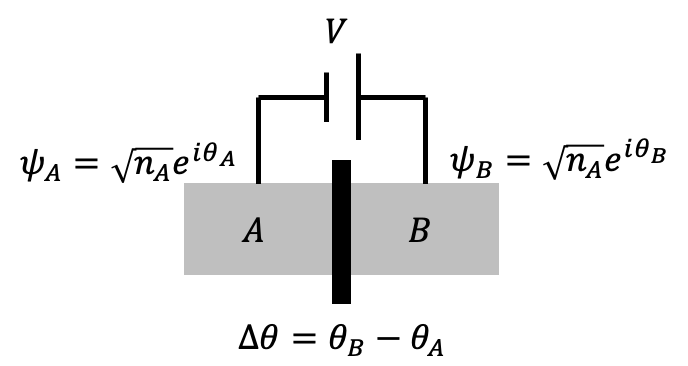
A Josephson junction can be described with its intrinsic properties represented by \(H_0\). When a voltage \(V\) is applied across the junction, the interaction between the superconducting wavefunctions is represented by \(K\). The equation of motion is given as: \[ i\hbar \frac{\partial}{\partial t} \begin{pmatrix} \sqrt{n_A} e^{i\theta_A} \\ \sqrt{n_B} e^{i\theta_B} \end{pmatrix} = \begin{pmatrix} H_0 - \frac{qV}{2} & K \\ K & H_0 + \frac{qV}{2} \end{pmatrix} \begin{pmatrix} \sqrt{n_A} e^{i\theta_A} \\ \sqrt{n_B} e^{i\theta_B} \end{pmatrix}. \] When \(q = -2e\) (Cooper pairs), the equation becomes: \[ i\hbar \frac{\partial}{\partial t} \begin{pmatrix} \sqrt{n_A} e^{i\theta_A} \\ \sqrt{n_B} e^{i\theta_B} \end{pmatrix} = \begin{pmatrix} H_0 + eV & K \\ K & H_0 - eV \end{pmatrix} \begin{pmatrix} \sqrt{n_A} e^{i\theta_A} \\ \sqrt{n_B} e^{i\theta_B} \end{pmatrix}. \]

Derivation for \(\theta_A, n_A\)

The first equation is: \[ i\hbar \frac{\partial}{\partial t} (\sqrt{n_A} e^{i\theta_A}) = \frac{i}{2} \frac{e^{i\theta_A}}{\sqrt{n_A}} \frac{\partial n_A}{\partial t} - \sqrt{n_A} e^{i\theta_A} \frac{\partial \theta_A}{\partial t} = (H_0 + eV) \sqrt{n_A} e^{i\theta_A} + K\sqrt{n_B} e^{i\theta_B}. \] Separating the real and imaginary parts gives: \[ \frac{i}{2}\hbar \frac{\partial n_A}{\partial t} - n_A \hbar \frac{\partial \theta_A}{\partial t} = (H_0 + eV)n_A + K\sqrt{n_A n_B} e^{i(\theta_B - \theta_A)}. \] Its conjugate equation is: \[ -\frac{i}{2}\hbar \frac{\partial n_A}{\partial t} - n_A \hbar \frac{\partial \theta_A}{\partial t} = (H_0 + eV)n_A + K\sqrt{n_A n_B} e^{-i(\theta_B - \theta_A)}. \]

Adding the two equations gives: \[ -2n_A \hbar \frac{\partial \theta_A}{\partial t} = 2(H_0 + eV)n_A + 2K\sqrt{n_A n_B} \cos(\theta_B - \theta_A), \] yielding the equation for \(\theta_A\): \[ \hbar \frac{\partial \theta_A}{\partial t} = -(H_0 + eV) - K\sqrt{\frac{n_B}{n_A}} \cos(\theta_B - \theta_A). \]
Subtracting the two equations gives: \[ i\hbar \frac{\partial n_A}{\partial t} = 2iK\sqrt{n_A n_B} \sin(\theta_B - \theta_A), \] which simplifies to: \[ \hbar \frac{\partial n_A}{\partial t} = 2K\sqrt{n_A n_B} \sin(\theta_B - \theta_A). \]

Derivation for \(\theta_B, n_B\)

The second equation is: \[ i\hbar \frac{\partial}{\partial t} (\sqrt{n_B} e^{i\theta_B}) = \frac{i}{2} \frac{e^{i\theta_B}}{\sqrt{n_B}} \frac{\partial n_B}{\partial t} - \sqrt{n_B} e^{i\theta_B} \frac{\partial \theta_B}{\partial t} = K\sqrt{n_A} e^{i\theta_A} + (H_0 - eV)\sqrt{n_B} e^{i\theta_B}. \] Separating this gives: \[ \frac{i}{2}\hbar \frac{\partial n_B}{\partial t} - n_B \hbar \frac{\partial \theta_B}{\partial t} = K\sqrt{n_A n_B} e^{-i(\theta_B - \theta_A)} + (H_0 - eV)n_B. \] Its conjugate equation is: \[ -\frac{i}{2}\hbar \frac{\partial n_B}{\partial t} - n_B \hbar \frac{\partial \theta_B}{\partial t} = K\sqrt{n_A n_B} e^{i(\theta_B - \theta_A)} + (H_0 - eV)n_B. \]

Adding the two equations gives: \[ -2n_B \hbar \frac{\partial \theta_B}{\partial t} = 2K\sqrt{n_A n_B} \cos(\theta_B - \theta_A) + 2(H_0 - eV)n_B, \] which simplifies to: \[ \hbar \frac{\partial \theta_B}{\partial t} = -(H_0 - eV) - K\sqrt{\frac{n_A}{n_B}} \cos(\theta_B - \theta_A). \]
Subtracting the two equations gives: \[ i\hbar \frac{\partial n_B}{\partial t} = -2iK\sqrt{n_A n_B} \sin(\theta_B - \theta_A), \] which simplifies to: \[ \hbar \frac{\partial n_B}{\partial t} = -2K\sqrt{n_A n_B} \sin(\theta_B - \theta_A). \]

Combining these results:

• For \(\theta_A\): \[ \hbar \frac{\partial \theta_A}{\partial t} = -(H_0 + eV) - K\sqrt{\frac{n_B}{n_A}} \cos(\theta_B - \theta_A). \]
• For \(\theta_B\): \[ \hbar \frac{\partial \theta_B}{\partial t} = -(H_0 - eV) - K\sqrt{\frac{n_A}{n_B}} \cos(\theta_B - \theta_A). \]
• For \(n_A\): \[ \hbar \frac{\partial n_A}{\partial t} = 2K\sqrt{n_A n_B} \sin(\theta_B - \theta_A). \]
• For \(n_B\): \[ \hbar \frac{\partial n_B}{\partial t} = -2K\sqrt{n_A n_B} \sin(\theta_B - \theta_A). \]

Defining the phase difference \(\Delta \theta = \theta_B - \theta_A\) and combining the first two equations, we find: \[ \hbar \frac{\partial \Delta \theta}{\partial t} = 2eV + \frac{K}{\hbar} \left( \frac{n_B - n_A}{\sqrt{n_A n_B}} \right) \cos\Delta \theta. \] Combining the last two equations and defining the current \(I\) as: \[ -\frac{\partial n_A}{\partial t} = \frac{\partial n_B}{\partial t} \equiv \frac{I}{-2e}, \] we obtain: \[ I = \frac{4eK}{\hbar} \sqrt{n_A n_B} \sin\Delta \theta \equiv I_c \sin\Delta \theta, \] where \(I_c\) is the critical current of the Josephson junction.

The nonlinear inductance of the Josephson junction is defined as: \[ L_J(\Delta \theta) = \left(\frac{2e}{\hbar I_c \cos\Delta \theta}\right). \] The energy stored in the inductance is: \[ E = \int IV dt = \int I_0 \sin\Delta \theta \cdot \frac{\hbar}{q} \frac{\partial \Delta \theta}{\partial t} dt = -\frac{I_0 \hbar}{2e} \cos\Delta \theta \equiv -\frac{I_0 \Phi_0}{2\pi} \cos\Delta \theta, \] where the flux quantum is \(\Phi_0 = \frac{2\pi\hbar}{2e}\), and: \[ E_J = \frac{I_0 \Phi_0}{2\pi}. \]

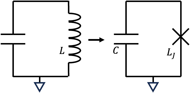
▲ Transforming a linear \(LC\) circuit into a nonlinear \(LC\) circuit by incorporating the nonlinear inductance of Josephson junctions. \(L_J\) represents the inductance of the Josephson junction.

Originally written in Chinese by the author, these articles are translated into English to invite cross-language resonance.