Qubit Physics

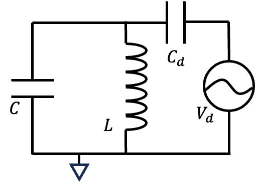
Now, let's discuss how to drive an LC circuit and a transmon qubit. By coupling the system to an external voltage source \( V_d \) through a coupling capacitor \( C_d \), the Lagrangian of the system is given by:

\[ \mathcal{L}_d(\dot{Q}, Q) = T - U = \frac{L\dot{Q}^2}{2} - \frac{Q^2}{2C} - \frac{Q_d^2}{2C_d} \]

The energy associated with the coupling capacitor \( C_d \) is:

\[ \frac{Q_d^2}{2C_d} = \frac{C_d (V - V_d)^2}{2} = \frac{C_d \left(\frac{Q}{C} - V_d\right)^2}{2} \] \[ = \frac{C_d Q^2}{2C^2} - \frac{C_d Q}{C}V_d + \frac{C_d V_d^2}{2} \]

Substituting the above expression into the Lagrangian and simplifying, we obtain:

\[ \mathcal{L}_d(\dot{Q}, Q) = \frac{L\dot{Q}^2}{2} - \frac{Q^2}{2C} - \frac{C_d}{C} \frac{Q^2}{2C} + \frac{C_d}{C} QV_d - \frac{C_d V_d^2}{2} \] \[ = \frac{L\dot{Q}^2}{2} - \frac{Q^2}{2C_\Sigma} + \frac{C_d}{C} QV_d - \frac{C_d V_d^2}{2} \]

Here, \( C_\Sigma = \frac{C^2}{C + C_d} \). We define the canonical momentum as:

\[ \Phi = -\frac{\partial \mathcal{L}_d}{\partial \dot{Q}} = -L\dot{Q} \quad \rightarrow \quad \dot{Q} = -\frac{\Phi}{L} \]

Next, we calculate the Hamiltonian:

\[ \bar{\mathcal{H}} _d = -\mathcal{L}_d - \Phi \dot{Q} = -\frac{L\dot{Q}^2}{2} + \frac{Q^2}{2C_\Sigma} - \frac{C_d}{C} QV_d + \frac{\Phi^2}{L} \] \[ = \frac{\Phi^2}{2L} + \frac{Q^2}{2C_\Sigma} - \frac{C_d}{C} QV_d \]

Detailed Derivation

Proceeding with canonical quantization:

\[ \begin{aligned} &a_d = \sqrt{\frac{1}{2\hbar} \sqrt{\frac{L}{C_\Sigma}}} \left(\sqrt{\frac{C_\Sigma}{L}} \Phi + iQ\right) \\ &a_d^\dagger = \sqrt{\frac{1}{2\hbar} \sqrt{\frac{L}{C_\Sigma}}} \left(\sqrt{\frac{C_\Sigma}{L}} \Phi - iQ\right) \end{aligned} \quad \leftrightarrow \quad \begin{aligned} &\Phi_d = \sqrt{\frac{\hbar}{2} \sqrt{\frac{L}{C_\Sigma}}} (a_d^\dagger + a_d) \\ &Q_d = i\sqrt{\frac{\hbar}{2} \sqrt{\frac{C_\Sigma}{L}}} (a_d^\dagger - a_d) \end{aligned} \]

Substituting these expressions, we obtain:

\[ = \hbar \sqrt{\frac{1}{LC_\Sigma}} \left( a_d^\dagger a_d + \frac{1}{2} \right) - \frac{C_d}{C} \sqrt{\frac{\hbar}{2 C_\Sigma \sqrt{LC_\Sigma}}} \cdot i (a_d^\dagger - a_d) V_d \]

Defining the frequency \( \omega_\Sigma = \frac{1}{\sqrt{L C_\Sigma}} \), we have:

\[ = \hbar \omega_\Sigma \left( a_d^\dagger a_d + \frac{1}{2} \right) - C_d V_d \sqrt{\frac{\omega_\Sigma}{2\hbar (C + C_d)}} \cdot i (a_d^\dagger - a_d) \]

The final result is:

\[ \bar{\mathcal{H}} _d = \hbar \omega_\Sigma \left(a_d^\dagger a_d + \frac{1}{2}\right) - i \Omega (a_d^\dagger - a_d) \]

Here, \( \Omega = C_d V_d \sqrt{\frac{\omega_\Sigma}{2\hbar (C + C_d)}} \) is known as the Rabi frequency.

Originally written in Chinese by the author, these articles are translated into English to invite cross-language resonance.