PHYS598500 · Week 2 · T2
超導電路量子化與 Transmon 設計
Circuit Quantization and Transmon Design
本週定位
W2 人工原子與 Transmon:五問主線
5 題
-
一個巨觀電路為什麼可能具有量子能階?
-
超導電路中,什麼東西扮演位置與動量?
-
為什麼最簡單的人工原子仍然不是 qubit?
-
Josephson junction 如何塑造人工原子的能階?
-
為什麼人工原子最後設計成 Transmon?
前言:我們能不能用電路製造一顆原子?
自然原子的離散能階來自電子在庫倫位能中的量子運動;超導量子位元則由電荷、磁通量與 Josephson phase 的量子運動形成。這一週不以公式推導作為故事主角,而是沿著一個問題前進: 如果自然原子的大小、頻率與能階幾乎不能由我們決定,我們能不能製造一顆可以自行設計的人工原子?
| 時間 | 問題 | 本段產出 |
|---|---|---|
| 0–10 分 | 人工原子開場與先備診斷 | 自然原子/電路人工原子的比較圖 |
| 10–30 分 | 問題一:巨觀電路的量子能階 | 巨觀量子相位與電路模式的概念鏈 |
| 30–50 分 | 問題二:電路的共軛變數 | \((\Phi,Q)\) 與 \((\varphi,n)\) 對照 |
| 50–70 分 | 問題三:LC oscillator 的限制 | 等間距能譜與不可選擇控制 |
| 70–95 分 | 問題四:Josephson nonlinearity | cosine potential 與 anharmonicity |
| 95–115 分 | 問題五:Transmon 的設計選擇 | charge dispersion/anharmonicity trade-off |
| 115–120 分 | Exit ticket 與逆向作業 | geometry → Hamiltonian 假說 |
問題一:一個巨觀電路為什麼可能具有量子能階?
「巨觀」不等於「必然古典」。超導體中的 Cooper pairs 形成具有共同相位的凝聚態;在低溫、低損耗與受控電磁環境下, 電路的集體模式可以保持足夠長的量子相干性。量子化的不是某一顆電子的位置,而是整個電路模式的電荷、磁通量與相位自由度。
先拆開一個常見誤解:粒子很多,不代表自由度一定很多
一塊超導金屬當然含有極大量的電子;但我們在低能量下不必逐一追蹤每顆電子。電子先形成 Cooper pairs, 再凝聚成一個具有長程相位關係的多體量子態。它可以用一個巨觀 order parameter 表示:
\[ \Psi(\mathbf r,t)=\sqrt{n_s(\mathbf r,t)}\,e^{i\theta(\mathbf r,t)}. \]
這裡 \(n_s\) 描述凝聚態密度,\(\theta\) 描述相位。絕對相位本身不是可觀測量;不同超導節點之間的 gauge-invariant phase difference 才會進入電流、磁通量與電路能量。也就是說,許多微觀粒子可以一起形成少數幾個 可控制的集體座標。真正要問的不是「電路裡有多少電子」,而是「低能量動力學最後剩下幾個獨立模式」。
類比而言,一根音叉也由大量原子組成,但最低振動可由一個 normal-mode amplitude 描述。超導電路的關鍵差別是: 這個集體模式可以在低溫與低損耗環境中進入量子極限,而不只表現為古典振動。
從巨觀相位到一個可以量子化的電路模式
超導體提供的並不只是「電阻等於零」。superconducting gap 抑制低能 quasiparticle excitation,凝聚態則提供相位剛性; 配合適當的電容、電感與邊界條件,整個電路可只留下少數低損耗的 electromagnetic modes。對其中一個模式,可先用 branch flux 作為座標:
\[ \Phi(t)\equiv\int^t V(t')\,dt', \qquad \varphi\equiv\frac{2\pi\Phi}{\Phi_0}, \qquad \Phi_0=\frac{h}{2e}. \]
電容儲存 electric energy,電感儲存 magnetic energy。若先看最簡單的單一 LC mode,它的 classical Hamiltonian 是
\[ H_{\rm mode}(\Phi,Q) =\frac{Q^2}{2C_{\rm eff}}+\frac{\Phi^2}{2L_{\rm eff}}, \qquad \omega=\frac{1}{\sqrt{L_{\rm eff}C_{\rm eff}}}. \]
第一項讓任意 charge accumulation 付出能量,第二項讓 flux 偏離平衡點時付出能量;兩者共同把這個自由度束縛成一個 normal mode。把這對電路變數提升為量子算符後,模式便成為 quantum harmonic oscillator:
\[ \hat H_{\rm mode} =\hbar\omega\left(\hat a^\dagger\hat a+\frac12\right), \qquad E_m=\hbar\omega\left(m+\frac12\right), \quad m=0,1,2,\ldots \]
這就是「巨觀電路具有離散量子能階」的最短存在性證明:先找到一個有 restoring energy 的集體模式,再量子化該模式。 問題二會正式回答 \(\Phi\) 與 \(Q\) 為何構成共軛變數;問題三則會追問:這串等間距能階為什麼仍然不能直接當作 qubit。
能階存在是一回事,實驗上看得見又是另一回事
形式上量子化之後一定有 \(E_m\);但若 thermal fluctuation 或環境造成的 linewidth 大於能階尺度,實驗只會看到近似連續的 古典響應。要讓最低幾個能階可辨認,至少需要
\[ k_BT\ll\hbar\omega, \qquad \hbar\kappa,\;\hbar\gamma_\phi\ll\hbar\omega, \]
其中 \(\kappa\) 是 mode energy decay rate,\(\gamma_\phi\) 是 dephasing rate。第一個條件抑制熱激發,後兩個條件避免 能階被 relaxation 與 phase noise 展寬到無法分辨。熱平衡下的平均 excitation number 為
\[ \bar n_{\rm th}=\frac{1}{e^{\hbar\omega/k_BT}-1}. \]
例如 \(f=\omega/2\pi=5\,\mathrm{GHz}\) 時,\(hf/k_B\approx0.24\,\mathrm{K}\)。若晶片模式真的熱化到 \(T=20\,\mathrm{mK}\),則 \(\bar n_{\rm th}\approx6\times10^{-6}\):系統幾乎都在 ground state。 實驗中仍須以 attenuation、filtering、shielding 與良好的封裝,避免 hot photons 與外界雜訊把有效溫度拉高。
為什麼日常電路看起來仍然是古典的?
日常 RLC circuit 並不是「沒有量子力學」,而是量子結構通常被三件事遮住:室溫使許多能階同時被佔據;電阻與環境耦合使 linewidth 變寬;強驅動又讓模式包含大量 quanta。對平均 photon number \(N=|\alpha|^2\gg1\) 的 coherent state, 相對 fluctuation 約按 \(1/\sqrt N\) 縮小,因此運動自然逼近 classical waveform。超導、稀釋製冷與 microwave engineering 的作用,就是把同一類電路推回 \(N\sim0,1\) 且 loss 足夠小的區域。
因此,一個巨觀電路能顯示量子能階,需要依序完成四個環節:
- 超導凝聚態與 Cooper-pair condensate:把大量電子組織成一個相位相干的低能多體態。
- 巨觀量子相位:讓不同節點之間的 phase difference 成為可進入電路動力學的集體變數。
- 低損耗電路與低溫環境:使 \(k_BT\) 與 energy linewidth 都小於 mode quantum \(\hbar\omega\)。
- 集體電路模式的量子化:由 circuit energy 找出 bounded normal mode,得到離散的 \(E_m\)。
核心判斷:電路是否具有量子能階,取決於它是否存在可辨認、可量子化並能與環境足夠隔離的集體自由度。 「具有離散能階」只完成了人工原子的第一步;能不能只選擇性控制其中兩階,則是後面三問要解決的設計問題。
單元 2:什麼是超導量子位元?
2.1 Artificial Atoms from Superconducting Circuits
超導量子位元可以被視為人工原子。 自然原子的能階來自電子在原子核庫倫位能中的量子化運動; 超導量子位元的能階則來自電路中電荷、磁通量與 Josephson phase 的量子化運動。
在古典 LC 電路中,能量在電容的電場能與電感的磁場能之間交換,形成諧振。 若把 LC 電路量子化,它會形成 quantum harmonic oscillator。 然而,理想 harmonic oscillator 的能階間距完全相等,無法單獨選取最低兩個能階作為 qubit。 因此,超導 qubit 必須引入非線性,使能階間距不再相等。
超導現象與 Josephson Junction
3.1 Superconductivity
超導是一種低溫量子凝聚態現象。當某些材料被冷卻到臨界溫度 \(T_c\) 以下時, 電阻消失,並且會排斥內部磁場,這稱為 Meissner effect。 在微觀層次中,電子透過與晶格振動的交互作用形成 Cooper pairs, 大量 Cooper pairs 進一步凝聚成具有共同相位的巨觀量子態。
超導體的重要特性
- Zero resistance:直流電阻消失,使電路耗散大幅降低。
- Meissner effect:超導體排斥磁場,形成磁通量屏蔽。
- Cooper pair condensate:電子成對凝聚,形成巨觀量子相干態。
- Macroscopic phase:超導態可用一個巨觀相位 \(\phi\) 描述。
- Flux quantization:超導迴路中的磁通量以 \(\Phi_0 = h/2e\) 為單位量子化。
3.2 Macroscopic Quantum Phase
超導凝聚態可以用一個巨觀波函數描述:
\[ \Psi({r}) = |\Psi({r})| e^{i\phi({r})} \]
其中 \(\phi\) 是超導相位。對超導量子電路而言, 這個相位不只是抽象變數,而是可以作為電路自由度並被量子化。 因此,超導量子電路中的重要變數通常包含電荷數 \(n\) 與相位 \(\varphi\), 並滿足類似位置與動量的共軛關係。
\[ [\hat{\varphi}, \hat{n}] = i \]
問題二:超導電路中,什麼東西扮演位置與動量?
機械系統以 position 與 momentum 描述狀態;電路則可用 node flux 與 node charge 描述。 Josephson circuit 中常改用 dimensionless phase \(\varphi\) 與 Cooper-pair number \(n\)。
第一步:不要把 voltage 當成 generalized coordinate
對一個電路節點,先選 ground 作為參考,定義 node voltage \(V(t)\)。但 Lagrangian mechanics 需要的是一個座標及其 time derivative,因此我們定義 node flux
\[ \Phi(t)\equiv\int_{-\infty}^{t}V(t')\,dt', \qquad \dot\Phi(t)=V(t). \]
名稱雖然叫 flux,它並不一定等於某個線圈內的磁通量;它首先是 voltage 的時間積分,單位同樣是 weber。 對連接節點 \(i,j\) 的 branch,branch flux 是 \(\Phi_i-\Phi_j\)。選定 spanning tree 與 ground 後, 獨立 node flux 就構成電路的 generalized coordinates。
第二步:從 LC energy 讀出 canonical momentum
對最簡單的平行 LC mode,capacitor voltage 是 \(\dot\Phi\),inductor current 是 \(\Phi/L\)。因此 electric energy 與 magnetic energy 分別為
\[ T=\frac12C\dot\Phi^2, \qquad U=\frac{\Phi^2}{2L}. \]
電路 Lagrangian 取 kinetic-like energy 減 potential-like energy:
\[ \mathcal L(\Phi,\dot\Phi) =\frac12C\dot\Phi^2-\frac{\Phi^2}{2L}. \]
與 \(\Phi\) 共軛的 canonical momentum 由定義直接算出:
\[ Q\equiv\frac{\partial\mathcal L}{\partial\dot\Phi} =C\dot\Phi=CV. \]
\(CV\) 正是 capacitor 上儲存的 charge。也就是說,node charge 不是靠類比猜出的「動量」; 它是從 circuit Lagrangian 對 \(\dot\Phi\) 微分後必然得到的 canonical momentum。
第三步:Legendre transform 得到 Hamiltonian
由 \(\dot\Phi=Q/C\),執行 Legendre transform:
\[ H(\Phi,Q) =Q\dot\Phi-\mathcal L =\frac{Q^2}{2C}+\frac{\Phi^2}{2L}. \]
因此機械 oscillator 與 LC oscillator 的對應不是只停在圖像類比,而是完整的 canonical mapping:
- \(x\longleftrightarrow\Phi\):描述系統偏離平衡點的 generalized coordinate。
- \(p\longleftrightarrow Q\):由 Lagrangian 對 generalized velocity 微分得到的 canonical momentum。
- \(m\longleftrightarrow C\):決定「動量項」\(Q^2/2C\) 的尺度。
- \(k\longleftrightarrow1/L\):決定 restoring potential \(\Phi^2/2L\) 的曲率。
第四步:canonical quantization
把 classical canonical pair 提升為 operators,並施加
\[ [\hat\Phi,\hat Q]=i\hbar, \qquad \Delta\Phi\,\Delta Q\geq\frac{\hbar}{2}. \]
在 flux representation 中,state 是 \(\psi(\Phi)\),而
\[ \hat\Phi\,\psi(\Phi)=\Phi\,\psi(\Phi), \qquad \hat Q\,\psi(\Phi)=-i\hbar\frac{\partial}{\partial\Phi}\psi(\Phi). \]
所以一個 state 若在 flux 上非常 localized,就必須包含很廣的 charge distribution;反之亦然。 這個 uncertainty relation 之後會成為 qubit design 的核心,而不是只有形式上的量子化規則。
第五步:Josephson circuit 改用 phase 與 Cooper-pair number
對超導節點,把有單位的 flux 與 charge 重新縮放:
\[ \varphi\equiv\frac{2\pi\Phi}{\Phi_0} =\frac{2e}{\hbar}\Phi, \qquad n\equiv\frac{Q}{2e}, \qquad \Phi_0=\frac{h}{2e}. \]
\(n\) 的正負會隨 branch orientation convention 改變;重要的是 \(2en\) 表示以 Cooper-pair charge 為單位的節點電荷。 代入上一個 commutator:
\[ [\hat\varphi,\hat n] =\frac{2e}{\hbar}\frac{1}{2e}[\hat\Phi,\hat Q] =i. \]
因而在 phase representation 中
\[ \hat n=-i\frac{\partial}{\partial\varphi}, \qquad e^{\pm i\hat\varphi}\ket n=\ket{n\pm1}. \]
最後一式把 phase 與 charge 的物理關係說得很清楚:\(e^{\pm i\hat\varphi}\) 會讓島上的 Cooper-pair number 改變一個單位。 因此 Josephson term 也可寫成
\[ -E_J\cos\hat\varphi =-\frac{E_J}{2}\left(e^{i\hat\varphi}+e^{-i\hat\varphi}\right), \]
它在 phase picture 是 cosine potential;在 charge picture 則是相鄰 charge states 之間的 coherent tunneling。 兩種圖像描述的是同一個 Hamiltonian。
因此 charge 與 phase 不能同時具有任意精確的值。後面所有 qubit 類型的差異,實際上都可視為在不同能量尺度下, 重新安排這一對共軛變數的 fluctuation、localization 與 sensitivity。較大的 charging energy 傾向限制 charge fluctuation, 較大的 Josephson energy 則傾向把 phase 限制在 cosine potential 的 minimum 附近;兩者不可能同時被任意壓窄。
問題二結論:超導電路中的「位置」是 node flux \(\Phi\) 或 dimensionless phase \(\varphi\); 對應的「動量」是 node charge \(Q\) 或 Cooper-pair number \(n\)。這不是命名習慣,而是由 \(\mathcal L(\Phi,\dot\Phi)\) 的 canonical structure 推導出來。
LC電路的正則量子化
簡諧振蕩
量子物理中常見的簡諧振蕩,經過量子化後能產生離散的能階,這正是量子計算基礎中的量子位元所依賴的概念。量子位元需要以具有量子效應的元件為基礎,利用超導體作為量子材料,結合 LC 振蕩電路的概念,製造出超導量子位元。本節將首先討論 LC 電路的量子化過程。
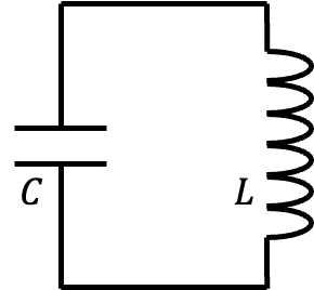
▲一個基礎的 \(LC\) 振蕩電路包含一個電感 \(L\) 和一個電容 \(C\)。定義電容攜帶的電荷為 \(Q\),當電容儲存的電荷改變速度(即 \(\dot{Q}\))時,即表示電路上的流動電流。電容和電感分別儲存的能量可表達為: \[ E_C = \frac{Q^2}{2C}, \quad E_L = \frac{L\dot{Q}^2}{2}. \] 我們可以將 \(E_L\) 視為動能項 \(T\),將 \(E_C\) 視為位能項 \(U\),從而定義拉格朗日量 \(L\): \[ \mathcal{L}(\dot{Q}, Q) = T - U = \frac{L\dot{Q}^2}{2} - \frac{Q^2}{2C}. \]
根據歐拉-拉格朗日方程: \[ \frac{d}{dt} \frac{\partial \mathcal{L}}{\partial \dot{Q}} - \frac{\partial \mathcal{L}}{\partial Q} = 0, \] 我們得到: \[ L\ddot{Q} + \frac{Q}{C} = 0 \implies \ddot{Q} + \frac{Q}{LC} = 0, \] 即描述一個以頻率 \(\omega = \frac{1}{\sqrt{LC}}\) 振蕩的簡諧運動。
量子化古典LC電路
什麼是正則量子化?
正則量子化是針對古典系統引入量子結構的一套方法,其核心是將 Hamiltonian 的 Poisson 結構替換為對易關係(commutator relation)。在前一節中,我們已經給出了 Lagrangian,現在透過 Lagendre 變換即可得到 Hamiltonian。
LC Circuit
LC 電路的基本關係
LC 電路由電容 \(C\) 與電感 \(L\) 組成。電容與電感的基本關係分別為: \[ \left\{ \begin{aligned} \text{Capacitor:}\qquad I_C &= C\frac{dV_C}{dt},\\[6pt] \text{Inductor:}\qquad V_L &= L\frac{dI_L}{dt}. \end{aligned} \right. \] 由於瞬時功率為 \(IV\),因此電路元件所儲存的能量可以寫成: \[ E=\int_{0}^{t}IV\,dt. \]
令 \(Q\) 表示電容上的電荷,則電路電流可以寫成 \(I=\dot{Q}\)。電容與電感所儲存的能量分別為: \[ \left\{ \begin{aligned} E_C &= \frac{Q^2}{2C},\\[6pt] E_L &= \frac{L\dot{Q}^{\,2}}{2}. \end{aligned} \right. \] 這組能量形式與質量-彈簧系統相對應: \[ \left\{ \begin{aligned} E_C &= \frac{Q^2}{2C},\\[6pt] E_L &= \frac{L\dot{Q}^{\,2}}{2} \end{aligned} \right. \quad\longleftrightarrow\quad \left\{ \begin{aligned} V &= \frac{1}{2}Kx^2,\\[6pt] T &= \frac{1}{2}m\dot{x}^{\,2}. \end{aligned} \right. \] 其中,\(x\) 為質量 \(m\) 的位移,\(K\) 為彈簧常數。兩個系統之間的對應關係為: \[ Q\longleftrightarrow x, \qquad L\longleftrightarrow m, \qquad \frac{1}{C}\longleftrightarrow K. \]
定義電感兩端的磁通量變數 \(\Phi\): \[ \Phi \equiv \int_{0}^{t}V_L\,dt = \int_{0}^{t} L\frac{dI_L}{dt}\,dt = LI_L = L\dot{Q}. \] 因為 LC 電路中的電容與電感具有相同的端電壓, \(V_L=V_C\),所以: \[ \frac{d\Phi}{dt} = V_L = V_C = \frac{Q}{C}. \] 因此,電荷 \(Q\) 與磁通量變數 \(\Phi\) 之間的關係為: \[ Q=C\dot{\Phi}. \]
將 \(Q=C\dot{\Phi}\) 以及 \(\Phi=L\dot{Q}\) 代入能量表達式,可以得到: \[ \left\{ \begin{aligned} E_C &= \frac{Q^2}{2C} = \frac{C\dot{\Phi}^{\,2}}{2},\\[8pt] E_L &= \frac{L\dot{Q}^{\,2}}{2} = \frac{\Phi^2}{2L}. \end{aligned} \right. \] 因此,以 \(\Phi\) 作為廣義座標時,電容能量扮演動能項,而電感能量扮演位能項。
LC 電路的 Lagrangian \(\mathcal{L}\) 為: \[ \mathcal{L} = E_C-E_L = \frac{C\dot{\Phi}^{\,2}}{2} - \frac{\Phi^2}{2L}. \]
與廣義座標 \(\Phi\) 對應的正則動量 \(\Pi\) 定義為: \[ \Pi \equiv \frac{\partial\mathcal{L}} {\partial\dot{\Phi}} = C\dot{\Phi} = Q. \] 因此,在 LC 電路中,磁通量 \(\Phi\) 的正則共軛動量就是電荷 \(Q\)。
Hamiltonian \(\mathcal{H}\) 由 Legendre transformation 定義為: \[ \mathcal{H} \equiv \Pi\dot{\Phi}-\mathcal{L}. \] 代入 \(\Pi=Q=C\dot{\Phi}\) 後,可以得到: \[ \mathcal{H} = \frac{Q^2}{2C} + \frac{\Phi^2}{2L}. \]
\[ [\hat{\Phi},\hat{Q}] = i\hbar \quad\longleftrightarrow\quad [x,p] = i\hbar. \]
正則座標的選擇 (Optional)
正則動量 \(\Phi_\#\) 定義為: \[ \Phi_\# \equiv \frac{\partial \mathcal{L}}{\partial \dot{Q}} = \mathcal{L}\dot{Q} \leftrightarrow \dot{Q} = \frac{\Phi_\#}{L}. \] 此處 \(\Phi_\#\) 的單位與磁通量相同,可以視為電感內部的磁通量。Hamiltonian \(H(\Phi_\#, Q)\) 定義為: \[ \mathcal{H} \equiv \Phi_\# \dot{Q} - \mathcal{L} = \frac{\Phi_\#^2}{2L} + \frac{Q^2}{2C}. \]
在量子系統中,正則座標 \(q\) 和正則動量 \(p\) 滿足對易關係: \[ [x, p] = i\hbar. \] 對於本文中的參數,量子化條件為: \[ [Q, \Phi_\#] = i\hbar. \]
本文目前採用 \(\Phi_\#\) 作為記號,這是因為與傳統文章採用的方式相反。傳統文章中,Hamiltonian 對於 \(\Phi_\#\) 與 \(Q\) 的地位是對稱的,定義誰是正則座標、誰是正則動量「似乎」是可以對換的(然而,Lagrangian 中動能和位能是反對稱的)。因此,本文直接反過來,將磁通量的部分作為廣義坐標,記為 \(\Phi\),而 \(Q\) 作為廣義動量。
在這種情況下,量子化條件變為: \[ [\Phi, Q] = i\hbar, \] 與本文的選擇差一個負號,即: \[ \Phi = -\Phi_\#. \] 這個負號也可以由 Lagrangian 的反對稱性進一步解釋。
有一種說法是因為後續會利用非線性的電感元件:約瑟夫森節(Josephson junction)取代線性電感,此非線性項如果出現在位能項比較好理解。不過,後面在驅動量子位元的時候,也是施加電容電壓來驅動,此時卻反而像驅動動能而不是驅動位能。以計算而言,誰是動能誰是位能是沒有差的。
我們引入新的變量 \(a\)、\(a^\dagger\): \[ a = \sqrt{\frac{1}{2\hbar} \sqrt{\frac{L}{C}}} \left( Q + i\sqrt{\frac{C}{L}} \Phi_\# \right), \quad a^\dagger = \sqrt{\frac{1}{2\hbar} \sqrt{\frac{L}{C}}} \left( Q - i\sqrt{\frac{C}{L}} \Phi_\# \right). \] 反之,可以表示為: \[ Q = \sqrt{\frac{\hbar}{2} \sqrt{\frac{C}{L}}} (a^\dagger + a), \quad \Phi_\# = i\sqrt{\frac{\hbar}{2} \sqrt{\frac{L}{C}}} (a^\dagger - a). \]
易證 \([a, a^\dagger] = 1\): \[ [a, a^\dagger] = aa^\dagger - a^\dagger a = \frac{1}{2\hbar} \sqrt{\frac{L}{C}} \left[ Q, \Phi_\# \right] = 1. \] 我們可以利用 \(a\)、\(a^\dagger\) 重寫 Hamiltonian \(H(\Phi_\#, Q)\): \[ \mathcal{H} = \frac{\Phi_\#^2}{2L} + \frac{Q^2}{2C} = \frac{\hbar \omega}{4} \left[ - (a^\dagger - a)^2 + (a^\dagger + a)^2 \right], \] 其中 \(\omega = \frac{1}{\sqrt{LC}}\)。 展開後可得: \[ \mathcal{H} = \frac{\hbar \omega}{2} \left[ a^\dagger a + a^\dagger a + 1 \right] = \hbar \omega \left[ a^\dagger a + \frac{1}{2} \right]. \]
最終得到量子化後的 Hamiltonian,每個能階差為 \(\hbar \omega\)。
動能與位能項的互換
正則座標的嚴格定義
實際上,要正確地透過對易關係(commutator relation)進行量子化,需要嚴格規定 \(x, p\) 的對應關係,否則可能會出現負號上的偏差。承接前一節,我們知道: \[ \dot{\Phi}_\# = \frac{d}{dt} \frac{\partial \mathcal{L}}{\partial \dot{Q}} = \frac{\partial \mathcal{L}}{\partial Q} = -\frac{Q}{C} \implies Q = -C\dot{\Phi}_\#. \] 現在,我們將 Lagrangian \(L\) 轉換到動量空間。
定義新的 Lagrangian \(\bar{\mathcal{L}}\) 為: \[ \bar{\mathcal{L}} \equiv \mathcal{L} - \frac{d}{dt} (\Phi_\# Q) = \mathcal{L} - \dot{\Phi}_\# Q - \Phi_\# \dot{Q}, \] 展開後可得: \[ \bar{\mathcal{L}} = \frac{L\dot{Q}^2}{2} - \frac{Q^2}{2C} - \dot{\Phi}_\# Q - \Phi_\# \dot{Q} = \frac{\Phi_\#^2}{2L} - \frac{C\dot{\Phi}_\#^2}{2} + C\dot{\Phi}_\#^2 - \frac{\Phi_\#^2}{L}, \] 簡化為: \[ \bar{\mathcal{L}} = \frac{C\dot{\Phi}_\#^2}{2} - \frac{\Phi_\#^2}{2L}. \]
注意,此時 \(\mathcal{L}(Q, \dot{Q}) \to \bar{\mathcal{L}}(\Phi_\#, \dot{\Phi}_\#)\),動能與位能的角色互換。同時,有 \(\bar{\mathcal{L}} = -\mathcal{L}\),對應於 Lagrangian 的反對稱性。為吸收這一反對稱性,我們定義新的變量: \[ \Phi = -\Phi_\#. \] 這使得: \[ \bar{\mathcal{L}}(\dot{\Phi}, \Phi) = \frac{C\dot{\Phi}^2}{2} - \frac{\Phi^2}{2L}. \]
對應的正則動量 \(\Pi\)(並利用前述結果與 \(Q\) 進行聯繫): \[ \Pi \equiv \frac{\partial \bar{\mathcal{L}}}{\partial \dot{\Phi}} = C\dot{\Phi} = -C\dot{\Phi}_\# = Q \implies \dot{\Phi} = \frac{\Pi}{C} = \frac{Q}{C}. \]
Hamiltonian \(\bar{\mathcal{H}}\) 定義為: \[ \bar{\mathcal{H}} = \Pi\dot{\Phi} - \bar{\mathcal{L}} = \frac{\Pi^2}{C} - \frac{\Pi^2}{2C} + \frac{\Phi^2}{2L} = \frac{\Pi^2}{2C} + \frac{\Phi^2}{2L}, \] 與先前的 \(\mathcal{H}\) 完全一致。此時的量子化條件為: \[ [\Phi, \Pi] = [\Phi, Q] = i\hbar, \] 與傳統條件相同。
定義新的變量 \(a\)、\(a^\dagger\): \[ a = \sqrt{\frac{1}{2\hbar} \sqrt{\frac{L}{C}}} \left( \sqrt{\frac{C}{L}} \Phi + iQ \right), \quad a^\dagger = \sqrt{\frac{1}{2\hbar} \sqrt{\frac{L}{C}}} \left( \sqrt{\frac{C}{L}} \Phi - iQ \right). \] 反之: \[ \Phi = \sqrt{\frac{\hbar}{2} \sqrt{\frac{L}{C}}} (a^\dagger + a), \quad Q = i\sqrt{\frac{\hbar}{2} \sqrt{\frac{C}{L}}} (a^\dagger - a). \]
易證 \([a, a^\dagger] = 1\): \[ [a, a^\dagger] = aa^\dagger - a^\dagger a = \frac{1}{2\hbar} \sqrt{\frac{L}{C}} \left[ \Phi, Q \right] = 1. \] Hamiltonian \(H(\Phi, Q)\) 可改寫為: \[ \mathcal{H} = \frac{\Phi^2}{2L} + \frac{Q^2}{2C} = \frac{\hbar}{4\sqrt{LC}} \left[ (a^\dagger + a)^2 - (a^\dagger - a)^2 \right]. \] 由於 \(\omega = \frac{1}{\sqrt{LC}}\),展開後可得: \[ \mathcal{H} = \frac{\hbar \omega}{4} \left[ (a^\dagger + a)^2 - (a^\dagger - a)^2 \right] = \hbar \omega \left[ a^\dagger a + \frac{1}{2} \right]. \]
最終,我們再次得到量子化後的 Hamiltonian,其中每個能階的差異為 \(\hbar \omega\)。
形式化 Lagrangian 動能與位能的互換
簡化推導步驟
從 \(L(\dot{Q}, Q)\) 出發,基於 Lagrangian 動能與位能的反對稱性,我們定義對應 \(\dot{Q}\) 的正則動量 \(\Phi\) 時手動加入一個負號,以吸收反對稱性(否則後續的 Hamiltonian 會為負): \[ \Phi \equiv -\frac{\partial \mathcal{L}}{\partial \dot{Q}} \implies \dot{\Phi} = -\frac{\partial \mathcal{L}}{\partial Q}. \] 接下來,我們將 Lagrangian 換到 \((\dot{\Phi}, \Phi)\) 空間,即動量空間的 Lagrangian \(\bar{\mathcal{L}}\): \[ \bar{\mathcal{L}} \equiv \mathcal{L} + \frac{d}{dt} (\Phi Q) = \mathcal{L} + \dot{\Phi} Q + \Phi \dot{Q}. \]
利用微分的方式,可以證明 \(\bar{\mathcal{L}} = \bar{\mathcal{L}}(\dot{\Phi}, \Phi)\) 是 \((\dot{\Phi}, \Phi)\) 空間的函數: \[ d\bar{\mathcal{L}} = d\mathcal{L} + d(\dot{\Phi} Q) + d(\Phi \dot{Q}) = \frac{\partial \mathcal{L}}{\partial \dot{Q}} d\dot{Q} + \frac{\partial \mathcal{L}}{\partial Q} dQ + Qd\dot{\Phi} + \dot{\Phi}dQ + \dot{Q}d\Phi + \Phi d\dot{Q}. \] 展開後,因為 \(-\Phi = \frac{\partial \mathcal{L}}{\partial \dot{Q}}\),我們有: \[ d\bar{\mathcal{L}} = -\Phi d\dot{Q} - \dot{\Phi} dQ + Q d\dot{\Phi} + \dot{\Phi} dQ + \dot{Q} d\Phi + \Phi d\dot{Q} = Q d\dot{\Phi} + \dot{Q} d\Phi. \]
此時,對應 \(\dot{\Phi}\) 的正則動量 \(\Pi\) 為: \[ \Pi = \frac{\partial \bar{\mathcal{L}}}{\partial \dot{\Phi}} = Q, \] 即與原來的 \(Q\) 相同。對應的 Hamiltonian \(\bar{\mathcal{H}}\) 定義為: \[ \bar{\mathcal{H}} = \Pi \dot{\Phi} - \bar{\mathcal{L}} = Q\dot{\Phi} - \mathcal{L} - \dot{\Phi} Q - \Phi \dot{Q} = -\mathcal{L} - \Phi \dot{Q}. \] 最終形式為: \[ \bar{\mathcal{H}}(Q, \Phi) = -\mathcal{L} - \Phi \dot{Q}. \]
這樣,我們可以簡化後續的推導,只需遵循以下步驟:
- 寫下 \(L(\dot{Q}, Q)\)。
- 定義 \(\Phi \equiv -\frac{\partial \mathcal{L}}{\partial \dot{Q}}\),並得到 \(\dot{Q}\) 與 \(\Phi\) 的關係。
- 直接求出對應的 Hamiltonian: \[ \bar{\mathcal{H}}(Q, \Phi) = -\mathcal{L} - \Phi \dot{Q}, \] 並將 \(\dot{Q}\) 代入前述關係式。
- 量子化條件: \[ [Q, \Phi] = i\hbar. \]
這樣無需經過繁瑣的轉換 \(L(\dot{Q}, Q) \to \bar{\mathcal{L}}(\dot{\Phi}, \Phi) \to \bar{\mathcal{H}}(Q, \Phi)\)。特別是在後續引入外力耦合項時(如在推導如何驅動與讀取量子位元時,外部訊號與量子位元交互作用,或是兩個量子位元之間的耦合),如果按照繁瑣的推導,會出現類似於電磁場下的動量 \(p \to p - eA\) 的情況,在中間轉換時極度複雜。
註:注意到: \[ \bar{\mathcal{H}}(Q, \Phi) = -\mathcal{L} - \Phi \dot{Q} = -\mathcal{L} + \frac{\partial \mathcal{L}}{\partial \dot{Q}} \dot{Q} = H(\Phi, Q). \] \(H(\Phi, Q)\) 就是傳統上熟悉的 Hamiltonian。同時,\(\bar{\mathcal{H}} = H\) 再一次表明了 Hamiltonian 動能與位能的對稱性。
進階主線:Circuit → Lagrangian → Hamiltonian → Spectrum
(W2-C1, W2-D1, W2-D2)對節點磁通 \(\Phi\) 而言,電容網路提供 kinetic term,電感與 Josephson junction 提供 potential term:
\[\mathcal L=\frac12\dot{\Phi}^{T} C\dot{\Phi}-U(\Phi),\qquad Q=\frac{\partial\mathcal L}{\partial\dot{\Phi}}\]
Legendre transform 得到 \(H(\Phi, Q)\),再施加 \([\hat\Phi_i,\hat Q_j]=i\hbar\delta_{ij}\)。線性 LC 電路只產生等距能階;Josephson term
\[U_J(\varphi)=-E_J\cos\varphi,\qquad E_J=\frac{\Phi_0 I_c}{2\pi}\]
才打破 harmonicity,使最低兩能階可以被選擇性控制。進階課需要讓學生實際走完一次「由 schematic 到 Hamiltonian」;只背 transmon 公式不足以判斷寄生 mode、coupling 與 layout 變更的後果。
邊界:本週不深入 BCS microscopic derivation;超導體在這裡主要提供 macroscopic phase、低損耗 wiring 與 Josephson element。微觀材料損耗留到 T6。
課堂整合與驗收
研討問題:由一個含 \(C\)、\(L\)、JJ 的單節點電路寫出 \(\mathcal L\)、canonical charge 與 \(H\),並指出哪個參數由版圖或製程控制。
完成條件:學生必須留下可檢查的推導、關係圖、比較表或 architecture decision,並能說明其物理假設與工程代價。
核心與延伸閱讀
- Introduction to Quantum Electromagnetic CircuitsU. Vool and M. H. Devoret, International Journal of Circuit Theory and Applications 45, 897–934 (2017).從電路圖、Lagrangian 到量子 Hamiltonian 的核心讀物。
- Black-box Superconducting Circuit QuantizationS. E. Nigg et al., Physical Review Letters 108, 240502 (2012).把分佈式電磁環境與 Josephson 非線性轉成有效 Hamiltonian。
- A Quantum Engineer's Guide to Superconducting QubitsP. Krantz et al., Applied Physics Reviews 6, 021318 (2019).控制、coherence、readout 與工程參數的主幹 review。
- Engineering High-Coherence Superconducting QubitsI. Siddiqi, Nature Reviews Materials 6, 875–891 (2021).不同 qubit architecture、材料損耗與 coherence 的設計 trade-off。
問題三:為什麼最簡單的人工原子仍然不是 qubit?
量子化的 LC circuit 已經具有離散能階:
\[ \hat H_{LC}=\frac{\hat Q^2}{2C}+\frac{\hat\Phi^2}{2L} =\hbar\omega\left(\hat a^\dagger\hat a+\frac12\right), \qquad \omega=\frac1{\sqrt{LC}}. \]
先確認:LC circuit 的確已經是量子系統
定義 characteristic impedance \(Z=\sqrt{L/C}\),可把 flux 與 charge operators 寫成
\[ \hat\Phi=\Phi_{\rm zpf}(\hat a+\hat a^\dagger), \qquad \hat Q=-iQ_{\rm zpf}(\hat a-\hat a^\dagger), \]
\[ \Phi_{\rm zpf}=\sqrt{\frac{\hbar Z}{2}}, \qquad Q_{\rm zpf}=\sqrt{\frac{\hbar}{2Z}}, \qquad \Phi_{\rm zpf}Q_{\rm zpf}=\frac{\hbar}{2}. \]
即使在 ground state,flux 與 charge 仍有 zero-point fluctuation。能量本徵態 \(\ket m\) 也是真正離散的:
\[ E_m=\hbar\omega\left(m+\frac12\right), \qquad m=0,1,2,\ldots \]
所以問題不在於 LC oscillator「不夠量子」。它的問題恰好相反:它是一個太理想的 linear quantum system, 每一階都遵循完全相同的規則。
等間距能譜使所有相鄰 transition 頻率重疊
相鄰能階的 transition frequency 是
\[ \omega_{m,m+1} =\frac{E_{m+1}-E_m}{\hbar} =\omega, \]
因此
\[ \omega_{01}=\omega_{12}=\omega_{23}=\cdots. \]
一個 resonant microwave tone 不只看見 \(\ket0\leftrightarrow\ket1\),也會看見更高階 transition。 頻率選擇無法告訴系統「只使用最低兩階」。
從 drive Hamiltonian 看見 leakage 為何不可避免
假設以電容耦合的 microwave voltage 驅動 oscillator。忽略不影響主旨的 coupling prefactor,可將控制項寫成
\[ \hat H_d(t) =\hbar\epsilon(t)(\hat a+\hat a^\dagger). \]
相鄰能階的 matrix element 為
\[ \langle m+1|\hat a+\hat a^\dagger|m\rangle =\sqrt{m+1}. \]
drive 一開始把 \(\ket0\) 推向 \(\ket1\);一旦 \(\ket1\) 有 population,同一個頻率又正好 resonant 地驅動 \(\ket1\rightarrow\ket2\),而且 matrix element 是 \(\sqrt2\) 倍。再往上依此類推。 因此 \(\{\ket0,\ket1\}\) 並不是在這個控制下封閉的 invariant subspace。
更強的說法:linear drive 產生 coherent state,不會產生純 \(\ket1\)
在 rotating-wave approximation 下,受驅 harmonic oscillator 可寫成
\[ \hat H_{\rm rot}(t) =\hbar\bigl[\epsilon(t)\hat a^\dagger+\epsilon^*(t)\hat a\bigr]. \]
若初態是 vacuum,任何這類 linear pulse 最後只會做 displacement:
\[ \ket0\longrightarrow\hat D(\alpha)\ket0=\ket\alpha, \qquad P_m=e^{-|\alpha|^2}\frac{|\alpha|^{2m}}{m!}. \]
想讓 \(P_1\) 最大時需取 \(|\alpha|^2=1\),但此時 \(P_1^{\rm max}=e^{-1}\approx0.368\),其餘 population 仍分散在 \(\ket0,\ket2,\ldots\)。 換句話說,對 bare harmonic oscillator 做一個傳統 qubit「\(\pi\)-pulse」並不能把 \(\ket0\) 確定地翻到 \(\ket1\)。
qubit 還需要 spectral addressability
定義 anharmonicity
\[ \alpha\equiv\omega_{12}-\omega_{01}. \]
harmonic oscillator 有 \(\alpha=0\)。若引入 nonlinearity 使 \(\alpha\neq0\),drive frequency 才能以 \(\omega_{01}\) 選中 computational transition,同時對 \(\omega_{12}\) 保持 off-resonant。對簡單 pulse, 通常希望
\[ |\alpha|\gg\Omega_R,\;\kappa,\;\gamma_\phi, \]
其中 \(\Omega_R\) 是 Rabi rate。drive 太快時頻寬變寬,leakage amplitude 通常按 \(\Omega_R/|\alpha|\) 的量級增加;drive 太慢又會累積 decoherence。這就是之後 pulse shaping 與 DRAG control 所處理的 speed–leakage trade-off。
精確說法:harmonic oscillator 不是不能承載量子資訊;利用多個 Fock states、cat states 或其他 bosonic encoding,仍可把 oscillator 當作 logical qubit。但若只允許一般 linear microwave control, bare LC oscillator 不能自然提供一個可獨立操作的最低兩能階 qubit。
課堂任務:畫出 harmonic 與 anharmonic spectrum,標示同一頻率的 drive 會連接哪些 transition。
問題三結論:「能階離散」只保證系統是量子的;「能階不等距」才讓 \(\ket0\leftrightarrow\ket1\) 能被頻率選擇,並把 leakage 壓到可控制的程度。
2.2 Why Nonlinearity Is Necessary
若量子電路的能階為等間距,則從 \(\ket{0}\) 到 \(\ket{1}\) 的頻率與 從 \(\ket{1}\) 到 \(\ket{2}\) 的頻率相同。 這會導致微波控制無法只針對 qubit 子空間 \(\ket{0}, \ket{1}\), 而容易激發到更高能階。
Josephson junction 提供了超導量子電路所需的非線性電感。 透過這個非線性,超導電路可以形成不等間距能階,使最低兩個能階能夠被用作量子位元。
4.1 From LC Circuit to Quantum LC Oscillator
在古典電路中,LC 振盪器的能量在電容與電感之間交換。 電容儲存電場能,電感儲存磁場能。 若將 LC 振盪器量子化,會得到等間距能階:
\[ E_m = \hbar\omega\left(m + \frac{1}{2}\right) \]
這樣的 harmonic oscillator 並不適合作為 qubit,因為相鄰能階間距相同, 控制脈衝無法只選擇 \(\ket{0} \leftrightarrow \ket{1}\) transition。
問題四:Josephson junction 如何塑造人工原子的能階?
Josephson tunneling 提供不耗散、由 phase 控制的非線性元件:
\[ I=I_c\sin\varphi, \qquad V=\frac{\Phi_0}{2\pi}\dot\varphi, \qquad U_J(\varphi)=-E_J\cos\varphi. \]
Josephson energy 不是另外假設的:它可由兩條 Josephson relations 積分得到
理想 junction 的 supercurrent branch 滿足 \(I=I_c\sin\varphi\),phase 隨 voltage 的演化則滿足 \(V=(\Phi_0/2\pi)\dot\varphi\)。流入元件的瞬時功率為
\[ P=IV =I_c\sin\varphi\, \frac{\Phi_0}{2\pi}\dot\varphi. \]
若這份功率儲存在 junction potential 中,則
\[ \frac{dU_J}{dt} =\frac{dU_J}{d\varphi}\dot\varphi =\frac{\Phi_0 I_c}{2\pi}\sin\varphi\,\dot\varphi. \]
因而
\[ \frac{dU_J}{d\varphi}=E_J\sin\varphi, \qquad E_J\equiv\frac{\Phi_0 I_c}{2\pi} =\frac{\hbar I_c}{2e}, \]
積分後得到
\[ U_J(\varphi)=-E_J\cos\varphi+\text{constant}. \]
所謂「Josephson junction 提供 cosine potential」,因此不是把電路硬套進某個原子模型,而是從可量測的 current–phase relation 直接導出的 energy landscape。
它像電感,但不是線性電感
對線性電感,\(I=\Phi/L\),所以 potential 永遠是 quadratic。對 junction, \(\dot I=I_c\cos\varphi\,\dot\varphi\)。比較 \(V=L_J\dot I\) 可得 differential inductance
\[ L_J(\varphi) =\frac{\Phi_0}{2\pi I_c\cos\varphi}. \]
\(L_J\) 隨 phase 改變,這就是 nonlinearity 的電路語言。小振幅且 \(\varphi\approx0\) 時, \(L_J(0)=\Phi_0/(2\pi I_c)\),junction 看起來近似線性;振幅增大後,\(\cos\varphi\) 的變化便不能忽略。 理想 Josephson supercurrent 同時又是不耗散的,這使 junction 能在低損耗電路中提供一般 resistor 或 semiconductor diode 難以兼得的強 nonlinearity。實際元件仍有 junction capacitance、quasiparticle loss 與材料缺陷,不能把「理想不耗散」誤解為完全沒有 loss。
加入 capacitance 後,phase 變成在 cosine potential 中運動的量子座標
將 junction 與總電容 \(C_\Sigma\) 合在一起,charging energy 定義為
\[ E_C\equiv\frac{e^2}{2C_\Sigma}. \]
Hamiltonian 成為
\[ \hat H =4E_C(\hat n-n_g)^2-E_J\cos\hat\varphi. \]
在「量子粒子」圖像中,\(\varphi\) 是 position,\(n\) 是 momentum;\(E_C\) 決定 kinetic-energy scale, \(E_J\) 則決定 periodic potential 的深度。改變 junction critical current 會改變 \(E_J\),改變 shunt capacitance 會改變 \(E_C\),所以這顆人工原子的「質量、束縛強度與能譜」都能由電路設計。
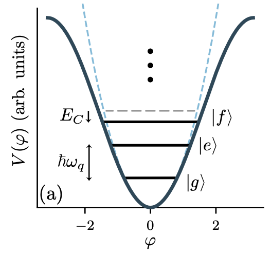
cosine 的 higher-order terms 破壞等間距
在線性化近似中只保留 potential minimum 附近的 quadratic term:
\[ -E_J\cos\varphi =-E_J+\frac{E_J}{2}\varphi^2 -\frac{E_J}{24}\varphi^4 +\frac{E_J}{720}\varphi^6-\cdots. \]
線性電感的 quadratic potential 只能產生 harmonic spectrum;Josephson junction 的 cosine potential 則提供 nonlinear inductance。 展開 cosine 時,quadratic term 建立主要振盪頻率,higher-order terms 破壞等間距,產生可供選擇控制的 anharmonic spectrum。
先把 quadratic part 當作 harmonic oscillator:
\[ \hat H_0 =4E_C\hat n^2+\frac{E_J}{2}\hat\varphi^2-E_J, \qquad \hbar\omega_p=\sqrt{8E_JE_C}. \]
對應的 zero-point amplitudes 可取為
\[ \hat\varphi=\varphi_{\rm zpf}(\hat a+\hat a^\dagger), \qquad \hat n=i n_{\rm zpf}(\hat a^\dagger-\hat a), \]
\[ \varphi_{\rm zpf} =\left(\frac{2E_C}{E_J}\right)^{1/4}, \qquad n_{\rm zpf} =\left(\frac{E_J}{32E_C}\right)^{1/4}, \qquad \varphi_{\rm zpf}n_{\rm zpf}=\frac12. \]
現在把 quartic term \(-E_J\hat\varphi^4/24\) 當作一階 perturbation。因為
\[ \langle m|(\hat a+\hat a^\dagger)^4|m\rangle =6m^2+6m+3, \]
得到低能階近似
\[ E_m\approx -E_J+\sqrt{8E_JE_C}\left(m+\frac12\right) -\frac{E_C}{12}(6m^2+6m+3). \]
因此相鄰 transition 不再等頻:
\[ \hbar\omega_{m,m+1} \approx\sqrt{8E_JE_C}-E_C(m+1), \]
\[ \hbar\omega_{01}\approx\sqrt{8E_JE_C}-E_C, \qquad \hbar\omega_{12}\approx\sqrt{8E_JE_C}-2E_C, \]
\[ \alpha\equiv\omega_{12}-\omega_{01} \approx-\frac{E_C}{\hbar}. \]
負號表示能階越高,相鄰間距越小。這個結果來自 cosine 的 negative quartic correction; 它正是讓 \(\omega_{01}\) drive 對 \(\omega_{12}\) 失諧、使最低兩階得以被選擇控制的來源。
同一個 cosine 在兩種 basis 中提供兩種直覺
- phase basis:\(-E_J\cos\varphi\) 是 periodic wells;\(E_J/E_C\) 越大,低能 wavefunction 越集中在某個 minimum 附近。
- charge basis:\(-E_J\cos\hat\varphi\) 連接 \(\ket n\) 與 \(\ket{n\pm1}\),使原本交叉的 charge-state energies 形成 avoided crossings。
問題四結論:Josephson junction 不是單純「再加一個電感」,而是把 quadratic potential 換成可由 \(E_J\) 設計的 cosine potential。quadratic part 決定主要頻率,quartic 與更高階項則製造 anharmonicity;人工原子的可控制能譜由此產生。
3.3 Josephson Junction
Josephson junction 是由兩個超導體中間夾著一層極薄絕緣層所構成的結構, 通常記為 SIS junction,也就是 superconductor-insulator-superconductor。 雖然中間是絕緣層,Cooper pairs 仍然可以透過量子穿隧效應通過 junction, 形成 Josephson current。
Josephson Relations
Josephson junction 的電流與相位差之間具有非線性關係:
\[ I = I_c \sin\varphi \]
當 junction 兩端存在電壓 \(V\) 時,相位差會隨時間演化:
\[ V = \frac{\Phi_0}{2\pi}\frac{d\varphi}{dt} \]
其中 \(\Phi_0 = h/2e\) 是超導磁通量量子。 Josephson energy 可寫為:
\[ E_J = \frac{\Phi_0 I_c}{2\pi} \]
3.4 Josephson Junction as a Nonlinear Inductor
Josephson junction 的關鍵價值在於它提供非線性電感。 一般線性電感的能量與相位近似呈二次關係; Josephson junction 的能量則為:
\[ U_J(\varphi) = -E_J \cos\varphi \]
這個 cosine potential 使得電路能階不再等間距, 因此能從量子振盪器中選出最低兩個能階作為 qubit。
核心觀念
沒有 Josephson junction,超導 LC 電路只是近似 harmonic oscillator; 有了 Josephson junction,電路才具有足夠非線性,可以形成可選址的量子二能階系統。
學習檢核
- Josephson junction 為什麼能讓 Cooper pairs 穿過絕緣層?
- Josephson current 與相位差之間的關係是什麼?
- 為什麼 Josephson junction 可被視為 nonlinear inductor?
約瑟夫森節的非線性電感性質
非線性使得精確控制量子位元成為可能
約瑟夫森接面的量子描述
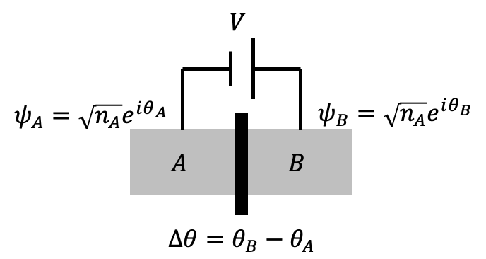
▲描述一個約瑟夫森接面,其材料的內秉性質由 \(H_0\) 描述。在接面兩端施加電壓 \(V\),超導波函數之間的交互作用以 \(K\) 表示,其運動方程為: \[ i\hbar \frac{\partial}{\partial t} \begin{pmatrix} \sqrt{n_A} e^{i\theta_A} \\ \sqrt{n_B} e^{i\theta_B} \end{pmatrix} = \begin{pmatrix} H_0 - \frac{qV}{2} & K \\ K & H_0 + \frac{qV}{2} \end{pmatrix} \begin{pmatrix} \sqrt{n_A} e^{i\theta_A} \\ \sqrt{n_B} e^{i\theta_B} \end{pmatrix}. \] 當 \(q = -2e\)(古柏對)時,方程變為: \[ i\hbar \frac{\partial}{\partial t} \begin{pmatrix} \sqrt{n_A} e^{i\theta_A} \\ \sqrt{n_B} e^{i\theta_B} \end{pmatrix} = \begin{pmatrix} H_0 + eV & K \\ K & H_0 - eV \end{pmatrix} \begin{pmatrix} \sqrt{n_A} e^{i\theta_A} \\ \sqrt{n_B} e^{i\theta_B} \end{pmatrix}. \]
\(\theta_A, n_A \)完整推導過程
第一條方程為: \[ i\hbar \frac{\partial}{\partial t} (\sqrt{n_A} e^{i\theta_A}) = \frac{i}{2} \frac{e^{i\theta_A}}{\sqrt{n_A}} \frac{\partial n_A}{\partial t} - \sqrt{n_A} e^{i\theta_A} \frac{\partial \theta_A}{\partial t} = (H_0 + eV) \sqrt{n_A} e^{i\theta_A} + K\sqrt{n_B} e^{i\theta_B}. \] 將實部與虛部分離後得到: \[ \frac{i}{2}\hbar \frac{\partial n_A}{\partial t} - n_A \hbar \frac{\partial \theta_A}{\partial t} = (H_0 + eV)n_A + K\sqrt{n_A n_B} e^{i(\theta_B - \theta_A)}. \] 其共軛方程為: \[ -\frac{i}{2}\hbar \frac{\partial n_A}{\partial t} - n_A \hbar \frac{\partial \theta_A}{\partial t} = (H_0 + eV)n_A + K\sqrt{n_A n_B} e^{-i(\theta_B - \theta_A)}. \]
| 將兩式相加可得: \[ -2n_A \hbar \frac{\partial \theta_A}{\partial t} = 2(H_0 + eV)n_A + 2K\sqrt{n_A n_B} \cos(\theta_B - \theta_A), \] 整理得到 \(\theta_A\) 的方程: \[ \hbar \frac{\partial \theta_A}{\partial t} = -(H_0 + eV) - K\sqrt{\frac{n_B}{n_A}} \cos(\theta_B - \theta_A). \] |
|---|
| 將兩式相減可得: \[ i\hbar \frac{\partial n_A}{\partial t} = 2iK\sqrt{n_A n_B} \sin(\theta_B - \theta_A), \] 即: \[ \hbar \frac{\partial n_A}{\partial t} = 2K\sqrt{n_A n_B} \sin(\theta_B - \theta_A). \] |
\(\theta_B, n_B \)完整推導過程
第二條方程為: \[ i\hbar \frac{\partial}{\partial t} (\sqrt{n_B} e^{i\theta_B}) = \frac{i}{2} \frac{e^{i\theta_B}}{\sqrt{n_B}} \frac{\partial n_B}{\partial t} - \sqrt{n_B} e^{i\theta_B} \frac{\partial \theta_B}{\partial t} = K\sqrt{n_A} e^{i\theta_A} + (H_0 - eV)\sqrt{n_B} e^{i\theta_B}. \] 拆分後為: \[ \frac{i}{2}\hbar \frac{\partial n_B}{\partial t} - n_B \hbar \frac{\partial \theta_B}{\partial t} = K\sqrt{n_A n_B} e^{-i(\theta_B - \theta_A)} + (H_0 - eV)n_B. \] 其共軛方程為: \[ -\frac{i}{2}\hbar \frac{\partial n_B}{\partial t} - n_B \hbar \frac{\partial \theta_B}{\partial t} = K\sqrt{n_A n_B} e^{i(\theta_B - \theta_A)} + (H_0 - eV)n_B. \]
| 將兩式相加可得: \[ -2n_B \hbar \frac{\partial \theta_B}{\partial t} = 2K\sqrt{n_A n_B} \cos(\theta_B - \theta_A) + 2(H_0 - eV)n_B, \] 整理得到 \(\theta_B\) 的方程: \[ \hbar \frac{\partial \theta_B}{\partial t} = -(H_0 - eV) - K\sqrt{\frac{n_A}{n_B}} \cos(\theta_B - \theta_A). \] |
|---|
| 將兩式相減可得: \[ i\hbar \frac{\partial n_B}{\partial t} = -2iK\sqrt{n_A n_B} \sin(\theta_B - \theta_A), \] 即: \[ \hbar \frac{\partial n_B}{\partial t} = -2K\sqrt{n_A n_B} \sin(\theta_B - \theta_A). \] |
整理得出以下方程:
- 對於 \(\theta_A\): \[ \hbar \frac{\partial \theta_A}{\partial t} = -(H_0 + eV) - K\sqrt{\frac{n_B}{n_A}} \cos(\theta_B - \theta_A). \]
- 對於 \(\theta_B\): \[ \hbar \frac{\partial \theta_B}{\partial t} = -(H_0 - eV) - K\sqrt{\frac{n_A}{n_B}} \cos(\theta_B - \theta_A). \]
- 對於 \(n_A\): \[ \hbar \frac{\partial n_A}{\partial t} = 2K\sqrt{n_A n_B} \sin(\theta_B - \theta_A). \]
- 對於 \(n_B\): \[ \hbar \frac{\partial n_B}{\partial t} = -2K\sqrt{n_A n_B} \sin(\theta_B - \theta_A). \]
定義相位差 \(\Delta \theta = \theta_B - \theta_A\),並將前兩個方程相減,可得: \[ \hbar \frac{\partial \Delta \theta}{\partial t} = 2eV + \frac{K}{\hbar} \left( \frac{n_B - n_A}{\sqrt{n_A n_B}} \right) \cos\Delta \theta. \] 將後兩條方程結合並定義電流 \(I\) 為: \[ -\frac{\partial n_A}{\partial t} = \frac{\partial n_B}{\partial t} \equiv \frac{I}{-2e}. \] 整理得到: \[ I = \frac{4eK}{\hbar} \sqrt{n_A n_B} \sin\Delta \theta \equiv I_c \sin\Delta \theta, \] 其中 \(I_c\) 為該約瑟夫森接面的臨界電流。
定義約瑟夫森接面的非線性電感: \[ L_J(\Delta \theta) = \left(\frac{2e}{\hbar I_c \cos\Delta \theta}\right). \] 電感儲存的能量為: \[ E = \int IV dt = \int I_0 \sin\Delta \theta \cdot \frac{\hbar}{q} \frac{\partial \Delta \theta}{\partial t} dt = -\frac{I_0 \hbar}{2e} \cos\Delta \theta \equiv -\frac{I_0 \Phi_0}{2\pi} \cos\Delta \theta, \] 其中,磁通量子 \(\Phi_0 = \frac{2\pi\hbar}{2e}\),並定義: \[ E_J = \frac{I_0 \Phi_0}{2\pi}. \]
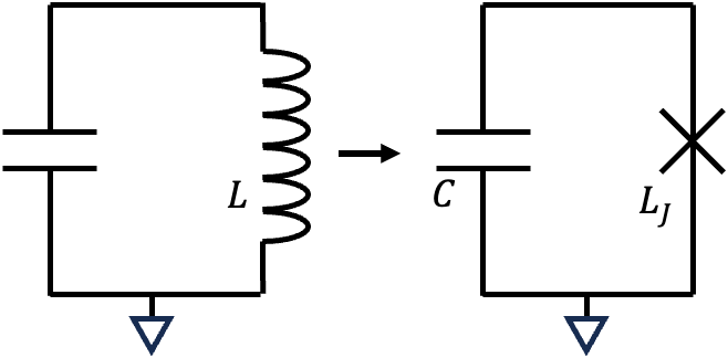
▲從線性的\(LC\)電路,變成以約瑟夫森節的非線性電感組合出的非線性\(LC\)電路。\(L_J\)為約瑟夫森節的電感值。
4.2 Nonlinear LC Circuit
Transmon 可以被理解為一個 nonlinear LC oscillator。 它以 Josephson junction 取代一般線性電感,並加入較大的 shunt capacitance。 Josephson junction 提供非線性,shunt capacitor 則降低 charging energy, 使 qubit 對 offset charge noise 不敏感。
Transmon 的基本電路包含:
- 一個 Josephson junction 或 SQUID loop。
- 一個大型 shunt capacitor。
- 與微波控制線、讀出共振腔或耦合器之間的電容耦合。
問題五:為什麼人工原子最後設計成 Transmon?
\[ \hat H_{\mathrm T}=4E_C(\hat n-n_g)^2-E_J\cos\hat\varphi. \]
Charge qubit 對 offset charge \(n_g\) 很敏感。Transmon 透過增加 shunt capacitance 降低 \(E_C\),提高 \(E_J/E_C\),使能量對 \(n_g\) 的 charge dispersion 指數受到壓低;代價是 anharmonicity 的絕對值減小, control selectivity 與 gate speed 之間必須重新取捨。
先看原始 charge qubit 的問題出在哪裡
在 charge basis 中,若先令 \(E_J=0\),每個整數 Cooper-pair number \(n\) 都對應一條 charging parabola:
\[ E_n(n_g)=4E_C(n-n_g)^2. \]
\(n_g\) 由 gate voltage、背景 trapped charge 與環境中的 offset-charge fluctuation 決定。 在 \(n_g=1/2\) 附近,只保留 \(\ket{n=0}\) 與 \(\ket{n=1}\) 時, Josephson tunneling 給出近似矩陣
\[ \hat H_{\{0,1\}} \approx \begin{pmatrix} 4E_Cn_g^2 & -E_J/2\\ -E_J/2 & 4E_C(1-n_g)^2 \end{pmatrix}. \]
因而兩能階 splitting 約為
\[ \hbar\omega_{01} \approx\sqrt{\bigl[4E_C(1-2n_g)\bigr]^2+E_J^2}. \]
在 \(n_g=1/2\) 正好有 charge sweet spot, \(\partial\omega_{01}/\partial n_g=0\);但只要工作點漂離 sweet spot,frequency 就會快速改變。 若背景 charge 發生跳動,qubit frequency 也跟著跳動。只靠精確 bias 在一個點上,並不是穩健的硬體保護。
Transmon 的硬體動作很簡單:把電容做大
對總電容 \(C_\Sigma\),
\[ E_C=\frac{e^2}{2C_\Sigma}. \]
加入大型 shunt capacitor 使 \(C_\Sigma\) 增加、\(E_C\) 降低,而 junction critical current 仍可獨立設定 \(E_J\)。 因此 \(E_J/E_C\) 可以由 charge-qubit regime 推向 \(E_J/E_C\gg1\) 的 transmon regime。 這不是換了一個 Hamiltonian,而是把同一個 Hamiltonian 移到另一個參數區。
在 phase picture 中,較大的 \(E_J/E_C\) 使 low-energy wavefunctions 集中在 cosine minimum 附近; 相鄰 wells 之間的 quantum phase slip amplitude 變小。offset charge \(n_g\) 在這個圖像中扮演 periodic potential 的 boundary phase,而 energy 對 \(n_g\) 的依賴正是由 inter-well tunneling 造成。 barrier 相對變高後,energy band 對 \(n_g\) 變平。
關鍵不只是「變小」,而是 charge dispersion 指數變小
在 \(E_J/E_C\gg1\) 的漸近區,能階對 offset charge 的主要依賴可寫成
\[ E_m(n_g)\approx\bar E_m -\frac{\epsilon_m}{2}\cos(2\pi n_g), \]
其中 charge-dispersion amplitude 的主導尺度為
\[ \epsilon_m \propto E_C\, \exp\!\left[-\sqrt{8E_J/E_C}\right] \times \text{algebraic prefactor}. \]
因而提高 \(E_J/E_C\) 時, \(\partial\omega_{01}/\partial n_g\) 不只是按 \(1/(E_J/E_C)\) 緩慢下降,而是得到 exponential suppression。 Transmon 的價值就在這個不對稱交換:用相對溫和的參數改動,換到非常強的 charge-noise dephasing suppression。
但 nonlinearity 沒有免費保留
問題四已得到
\[ \hbar\omega_{01}\approx\sqrt{8E_JE_C}-E_C, \qquad \alpha\equiv\omega_{12}-\omega_{01} \approx-\frac{E_C}{\hbar}. \]
shunt capacitance 使 \(E_C\) 下降,因此 \(|\alpha|\) 也近似線性下降。所幸 charge dispersion 是 exponential suppression,而 anharmonicity 只按 \(E_C\) 線性減小;於是存在一段實用的參數窗: charge noise 已經很弱,但 \(\omega_{01}\) 與 \(\omega_{12}\) 仍分得開。
對指定的 transition frequency 與 anharmonicity,這兩個近似式也可反過來作 first-pass design:
\[ \frac{E_C}{h}\approx\frac{|\alpha|}{2\pi}, \qquad \frac{E_J}{E_C} \approx\frac18 \left(\frac{hf_{01}+E_C}{E_C}\right)^2. \]
實際設計仍需 numerical diagonalization、junction fabrication model 與 electromagnetic simulation, 但這兩式已能顯示 pad capacitance、junction critical current、frequency 與 leakage 之間的方向關係。
保護沒有把控制一起關掉
capacitive microwave drive 主要透過 \(\hat n\) 耦合。在 harmonic approximation 中
\[ |\langle0|\hat n|1\rangle| \approx \left(\frac{E_J}{32E_C}\right)^{1/4}\neq0. \]
所以 \(E_J/E_C\) 增大時,charge dispersion 被壓低,但 \(0\leftrightarrow1\) electric-dipole matrix element 並沒有一起消失。這讓 transmon 同時保留成熟的 microwave drive 與 dispersive readout。 反面是:同一個非零 matrix element 也表示 transmon 並沒有自動免疫所有 high-frequency electric noise; 它主要解決的是低頻 offset-charge dephasing,而不是全面的 relaxation protection。
fixed-frequency 與 tunable transmon 是下一層交換
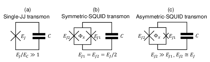
單一 junction 給 fixed \(E_J\),結構較簡單,也沒有額外 flux-noise channel;代價是 fabrication variation 直接變成 frequency spread,可能造成 frequency collision。若用對稱 dc SQUID 取代單一 junction,則
\[ E_{J,\mathrm{eff}}(\Phi_{\rm ext}) =2E_{J0} \left|\cos\!\left(\pi\frac{\Phi_{\rm ext}}{\Phi_0}\right)\right|, \]
qubit frequency 因而可調,可避開 collision 或執行 flux-mediated gate;但離開 flux sweet spot 後, \(\partial\omega_{01}/\partial\Phi_{\rm ext}\neq0\),flux noise、control-line crosstalk 與 calibration 負擔也隨之增加。
用四項設計判準重新看 Transmon
- Dephasing protection:\(\partial\omega_{01}/\partial n_g\) 因 charge dispersion 而受到 exponential suppression。
- Relaxation protection:不具一般性的 \(\langle0|\hat O_{\rm noise}|1\rangle\approx0\);材料 loss、Purcell loss 與高頻 electric noise 仍須另外工程化。
- Controllability:\(\langle0|\hat n|1\rangle\neq0\),保留有效的 microwave control 與 readout coupling。
- Leakage suppression:\(\Delta_{\rm leakage}\sim\hbar|\alpha|\) 有限;必須在 gate speed、pulse shaping 與剩餘 anharmonicity 間取捨。
- 得到:較低 charge dispersion、成熟的 microwave control、可設計的頻率範圍。
- 付出:較弱 anharmonicity、可能的 leakage、fixed/tunable design 的不同 noise 與 calibration 負擔。
- 設計觀念:Transmon 不是「最好的人造原子」,而是一組在 noise sensitivity、control 與製造可行性之間成功的參數選擇。
本週結論:具有離散能階還不等於 qubit;必須利用 Josephson nonlinearity 製造可選擇控制的能譜, 再利用 \(E_J/E_C\) 調整 charge sensitivity 與 anharmonicity 的交換。Transmon 之所以成為主流,不是因為它把所有 noise 都消除,而是因為它利用 exponential-versus-linear scaling 找到一個特別有效、又仍可控制與製造的 Pareto point。
既有推導與延伸教材
Transmon的性質
當前主流的超導量子位元
Ref:
DOI:10.48550/arXiv.2203.04164
單元 4:Transmon Qubit
4.3 Transmon Hamiltonian
Transmon Hamiltonian 可寫為:
\[ \hat{H}_{\mathrm{transmon}} = 4E_C(\hat{n} - n_g)^2 - E_J\cos\hat{\varphi} \]
其中:
- \(\hat{n}\):Cooper pair number operator。
- \(\hat{\varphi}\):Josephson junction 兩端的超導相位差。
- \(n_g\):offset charge,代表環境電荷雜訊或 gate-induced charge。
- \(E_C = e^2 / 2C_\Sigma\):charging energy,由總電容 \(C_\Sigma\) 決定。
- \(E_J = \Phi_0 I_c / 2\pi\):Josephson energy,由 junction critical current 決定。
Transmon 的重要設計條件是:
\[ \frac{E_J}{E_C} \gg 1 \]
在這個 regime 中,能階對 offset charge \(n_g\) 的敏感度會被大幅壓低, 但仍保留足夠的 anharmonicity,使最低兩個能階可以作為 qubit 使用。
4.4 Energy Spectrum and Anharmonicity
在 \(E_J/E_C \gg 1\) 的近似下,Transmon 的最低能階可近似為弱非諧振盪器。 其 \(\ket{0} \rightarrow \ket{1}\) transition frequency 約為:
\[ \omega_{01} \approx \frac{\sqrt{8E_JE_C} - E_C}{\hbar} \]
Transmon 的 anharmonicity 約為:
\[ \alpha = \omega_{12} - \omega_{01} \approx -\frac{E_C}{\hbar} \]
Anharmonicity 是量子閘控制中的重要參數。 若 \(|\alpha|\) 太小,微波脈衝容易造成 leakage 到 \(\ket{2}\); 若 \(|\alpha|\) 太大,通常代表 \(E_C\) 較大,可能提高對 charge noise 的敏感度。 因此 Transmon 設計需要在 charge-noise protection 與 control selectivity 之間取得平衡。
4.5 Design of \(E_C\) and \(E_J\)
Transmon 的設計核心在於選擇合適的 \(E_C\)、\(E_J\) 與 \(E_J/E_C\)。 這些參數分別由晶片幾何、材料與 Josephson junction 製程決定。
| 參數 | 定義 | 由什麼決定 | 設計影響 |
|---|---|---|---|
| \(E_C\) | \(e^2/2C_\Sigma\) | 總電容、pad 面積、耦合電容、封裝環境 | 決定 anharmonicity 與 charge-noise sensitivity |
| \(E_J\) | \(\Phi_0 I_c/2\pi\) | Josephson junction 面積、氧化層厚度、臨界電流密度 | 決定 qubit frequency 與 potential depth |
| \(E_J/E_C\) | Josephson energy 與 charging energy 比值 | junction 與 capacitor 的共同設計 | 控制 charge dispersion 與 anharmonicity 的 trade-off |
4.6 Fixed-Frequency and Tunable Transmon
Transmon 可以分為 fixed-frequency transmon 與 tunable transmon。 Fixed-frequency transmon 使用單一 Josephson junction,頻率在製作後大致固定。 Tunable transmon 則使用 SQUID loop 取代單一 junction,使有效 Josephson energy 可由外加磁通量調控。
\[ E_J(\Phi_{\mathrm{ext}}) \approx E_{J,\mathrm{max}} \left| \cos\left(\pi\frac{\Phi_{\mathrm{ext}}}{\Phi_0}\right) \right| \]
Tunable transmon 提供更高的控制彈性,可用於頻率調諧、兩量子位元閘與避免 frequency collision; 但同時也會增加對 flux noise 的敏感度。
設計直覺
Transmon 的成功來自一個簡潔但深刻的設計策略: 用較大的電容降低 \(E_C\),犧牲部分 anharmonicity, 換取對電荷雜訊的指數級保護。
學習檢核
- 為什麼單純的量子 LC oscillator 不適合作為 qubit?
- Josephson junction 在 Transmon 中扮演什麼角色?
- 為什麼 Transmon 需要設計在 \(E_J/E_C \gg 1\) 的區域?
- \(E_C\) 太大或太小分別會造成什麼問題?
- Fixed-frequency Transmon 與 Tunable Transmon 的優缺點為何?
進階主線:設計不是把 \(E_J/E_C\) 做得越大越好
\[H=4E_C(\hat n-n_g)^2-E_J\cos\hat\varphi\]
在 \(E_J/E_C\gg1\) 的 transmon regime,低能階近似
\[\hbar\omega_{01}\approx\sqrt{8E_JE_C}-E_C,\qquad \alpha\equiv\omega_{12}-\omega_{01}\approx-\frac{E_C}{\hbar}\]
charge dispersion 隨 \(\exp[-\sqrt{8E_J/E_C}]\)(帶有能階依賴的代數前因子)指數下降,但 anharmonicity 只以較慢尺度下降。這是 transmon 成功的核心;代價是 pulse selectivity、leakage、frequency crowding 與 fabrication spread 必須一起設計。
固定頻率 transmon 減少 flux-noise sensitivity;SQUID transmon 提供可調頻率與 gate mechanism,卻引入 flux line、sweet spot 與 drift 問題。真正的設計問題是 noise、control、coupling、yield 與 calibration 的聯立最佳化。
雙約瑟夫森節(SQUID)的非線性電感性質
頻率可調式量子位元
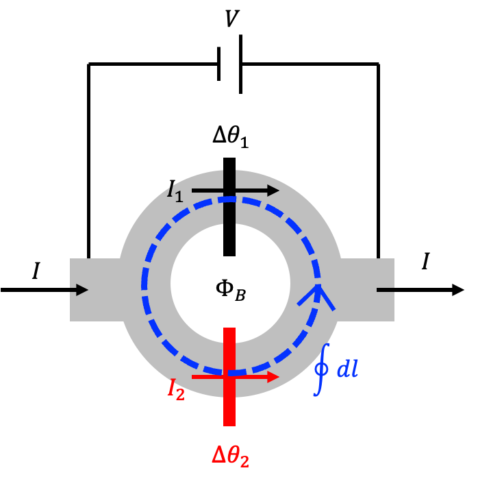
將兩組約瑟夫森節 \(J_1\)、\(J_2\) 相組,中間形成一個閉環,通入磁通 \( \Phi_B \) 與電壓 \( V \)。在前一節中,超導函數的相位對閉環的積分需滿足: \[ \oint \nabla \theta(r) \cdot d\vec{l} - \frac{q}{\hbar} \Phi_B = 2\pi N \] 因為在接面不連續會貢獻 \( \Delta\theta_1 \)、\( \Delta\theta_2 \),\( q = -2e \),帶入得: \[ \Delta\theta_2 - \Delta\theta_1 + 2\pi \frac{\Phi_B}{\Phi_0} = 2\pi N \] \[ \Delta\theta_2 = \Delta\theta_1 - 2\pi \frac{\Phi_B}{\Phi_0} + 2\pi N \]
當整個 SQUID 通入電流 \( I = I_1 + I_2 \),並使用前一節約瑟夫森節電流的關係式(這裡考慮對稱的 SQUID,即兩個約瑟夫森節的特性 \( I_c \) 相同),計算得: \[ I = I_1 + I_2 = I_0 (\sin\Delta\theta_1 + \sin\Delta\theta_2) \] \[ I = I_0 \left[\sin\Delta\theta_1 + \sin\left(\Delta\theta_1 - 2\pi \frac{\Phi_B}{\Phi_0} + 2\pi N\right)\right] \] \[ I = I_0 \left[\sin\Delta\theta_1 + \sin\left(\Delta\theta_1 - 2\pi \frac{\Phi_B}{\Phi_0}\right)\right] \] 利用三角恆等式化簡: \[ I = I_0 \left[2 \sin\left(\frac{\Delta\theta_1 + \Delta\theta_1 - 2\pi \frac{\Phi_B}{\Phi_0}}{2}\right) \cos\left(\frac{\Delta\theta_1 - \Delta\theta_1 + 2\pi \frac{\Phi_B}{\Phi_0}}{2}\right)\right] \] \[ I = 2I_0 \cos\left(\frac{\Phi_B}{\Phi_0} \pi\right) \sin\left(\Delta\theta_1 - \frac{\Phi_B}{\Phi_0} \pi\right) \]
前一節提到約瑟夫森節具有電感的性質,同理我們可以討論 SQUID 的電感性質。將電流對時間微分: \[ \dot{I} = 2I_0 \cos\left(\frac{\Phi_B}{\Phi_0} \pi\right) \cos\left(\Delta\theta_1 - \frac{\Phi_B}{\Phi_0} \pi\right) \dot{\Delta\theta_1} \] 而 \( \dot{\Delta\theta_1} \) 與電壓 \( V \) 的關係為: \[ V = \frac{\hbar}{2e} \dot{\Delta\theta_1} = \frac{\Phi_0}{2\pi} \dot{\Delta\theta_1} \] 帶入後可得電感值: \[ L_{\text{SQUID}}(\Delta\theta_1, \Phi_B) = \left[\frac{2\pi}{\Phi_0} \cdot 2I_0 \cos\left(\frac{\Phi_B}{\Phi_0} \pi\right) \cos\left(\Delta\theta_1 - \frac{\Phi_B}{\Phi_0} \pi\right)\right] \]
可以注意到 \( L_{\text{SQUID}} \) 的值會受到外加磁通 \( \Phi_B \) 的影響,這為後來 Tunable Transmon 調整頻率的關鍵。定義變數 \( \Phi \): \[ \Phi \equiv \frac{\Delta\theta_1}{\pi} \Phi_0 - \Phi_B = \frac{\Phi_0}{\pi} \left(\Delta\theta_1 - \frac{\Phi}{\Phi_0} \pi\right) \] 並有: \[ \dot{\Phi} = \frac{\Phi_0}{\pi} \dot{\Delta\theta_1} \] 電壓 \( V \) 和電流 \( I \) 分別為: \[ V = \frac{1}{2} \dot{\Phi}, \quad I = 2I_0 \cos\left(\frac{\Phi_B}{\Phi_0} \pi\right) \sin\left(\frac{\Phi}{\Phi_0} \pi\right) \]
固定外場 \( \Phi_B \) 下,一組 SQUID 儲存的能量為: \[ E = \int IV \, dt = \int \left[2I_0 \cos\left(\frac{\Phi_B}{\Phi_0} \pi\right) \sin\left(\frac{\Phi}{\Phi_0} \pi\right) \cdot \frac{1}{2} \dot{\Phi}\right] dt \] 化簡得: \[ E = I_0 \cos\left(\frac{\Phi_B}{\Phi_0} \pi\right) \int \sin\left(\frac{\Phi}{\Phi_0} \pi\right) d\Phi \] \[ E = -\frac{I_0 \Phi_0}{\pi} \cos\left(\frac{\Phi_B}{\Phi_0} \pi\right) \cos\left(\frac{\pi}{\Phi_0} \Phi\right) \]
Tunable Transmon
可調頻率的Transmon
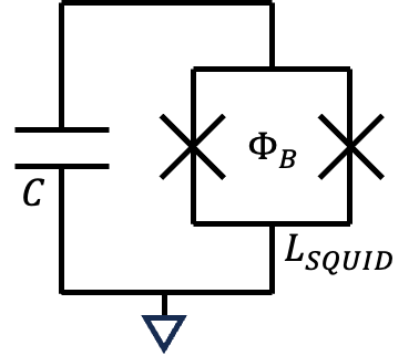
▲由兩個約瑟夫森節組合成可調電感值的\(LC\)電路。
前文提及約瑟夫森節具有電感性質,Transmon即是LC電路中的電感替換成約瑟夫森節。本節直接討論 Tunable Transmon,採用 SQUID 當作電感。實務上因為材料製作的不均一性,不同 Transmon 會有不一樣的特性,如果採用 Tunable Transmon,可以透過微調磁通量 \( \Phi_B \) 的方式使 Qubit 性質一致。此外,我們在前面量子化 LC 電路時,\([ \Phi, Q ] = i\hbar\) 是一對正則變量,利用 SQUID 的推導可以很自然地將磁通量 \( \Phi \) 與相位差 \( \Delta\theta \) 做聯繫,即: \[ \Phi \equiv \frac{\Delta\theta_1}{\pi} \Phi_0 - \Phi_B \]
現在我們寫下 Hamiltonian: \[ \mathcal{H} = \frac{Q^2}{2C} + \frac{\Phi_\#^2}{2L} = \frac{Q^2}{2C} + \frac{(I_0 \pi)}{2\Phi_0} \cos\left(\frac{\Phi_B}{\Phi_0} \pi\right) \Phi^2 - \frac{I_0}{24} \left(\frac{\pi}{\Phi_0}\right)^3 \cos\left(\frac{\Phi_B}{\Phi_0} \pi\right) \Phi^4 + \cdots \] \[ = \frac{Q^2}{2C} + \frac{\Phi^2}{2L} - \frac{1}{24L} \left(\frac{\pi}{\Phi_0}\right)^2 \Phi^4 + \cdots \] 其中: \[ L = \left(\frac{I_0 \pi}{\Phi_0} \cos\left(\frac{\Phi_B}{\Phi_0} \pi\right)\right)^{-1} \]
現在我們要討論非線性對於能階的改變,前文我們選擇新的變量 \( a \)、\( a^\dagger \): \[ a = \sqrt{\frac{1}{2\hbar} \sqrt{ \frac{L}{C}}} \left(\sqrt{\frac{C}{L}} \Phi + iQ\right), \quad a^\dagger = \sqrt{\frac{1}{2\hbar} \sqrt{ \frac{L}{C}}} \left(\sqrt{\frac{C}{L}} \Phi - iQ\right) \] 反之: \[ \Phi = \sqrt{\frac{\hbar}{2 }\sqrt{ \frac{L}{C}}} (a^\dagger + a), \quad Q = i\sqrt{\frac{\hbar}{2} \sqrt{ \frac{C}{L}}} (a^\dagger - a) \]
將 Hamiltonian 表達式展開為: \[ \mathcal{H} = \frac{\hbar}{\sqrt{LC}} \left[a^\dagger a + \frac{1}{2}\right] - \frac{1}{24L} \left(\frac{\pi}{\Phi_0}\right)^2 \left[i \sqrt{\frac{\hbar}{2\sqrt{L/C}}} (a^\dagger + a)\right]^4 \] 化簡後: \[ \mathcal{H} = \frac{\hbar}{\sqrt{LC}} \left[a^\dagger a + \frac{1}{2}\right] - \frac{\hbar^2}{96C} \left(\frac{\pi}{\Phi_0}\right)^2 (a^\dagger + a)^4 \] 該表達式包含線性和非線性項,線性項描述的是量子簡諧振子的能階,而非線性項源自於 Josephson 節對於能階的修正。
利用微擾理論,當 \( \mathcal{H} = H_0 + \Delta H \), \( \ket{E_0^m} \to \ket{E^m} \)、 \( E_0^m \to E^m = E_0^m + \delta E^m \),我們知道對能階 \( E_0^m \) 的修正 \( \delta E^m \) 為:
\[ \delta E^m = \langle E_0^m | \Delta H | E_0^m \rangle = \langle E_0^m | \left[-\frac{\hbar^2}{96C} \left(\frac{\pi}{\Phi_0}\right)^2 (a^\dagger + a)^4\right] | E_0^m \rangle \]
計算如下:
\[ \langle E_0^m | (a^\dagger + a)^4 | E_0^m \rangle = \langle E_0^m | (aa + aa^\dagger + a^\dagger a + a^\dagger a^\dagger)^2 | E_0^m \rangle \]
展開為:
\[ \langle E_0^m | aa(aa + aa^\dagger + a^\dagger a + a^\dagger a^\dagger) + aa^\dagger(aa + aa^\dagger + a^\dagger a + a^\dagger a^\dagger) + a^\dagger a(aa + aa^\dagger + a^\dagger a + a^\dagger a^\dagger) + a^\dagger a^\dagger(aa + aa^\dagger + a^\dagger a + a^\dagger a^\dagger) \ket{ E_0^m } \]
因為取期望值,只會留下 \( a, a^\dagger \) 次數相等的項,剩下:
\[ \langle E_0^m | aaa^\dagger a^\dagger + aa^\dagger aa^\dagger + aa^\dagger a^\dagger a + a^\dagger aaa^\dagger + a^\dagger aa^\dagger a + a^\dagger a^\dagger aa | E_0^m \rangle \]
繼續簡化:
\[ \langle E_0^m | a(a^\dagger a + 1)a^\dagger + aa^\dagger aa^\dagger + (a^\dagger a + 1)a^\dagger a + a^\dagger a(a^\dagger a + 1) + a^\dagger aa^\dagger a + a^\dagger (aa^\dagger - 1)a | E_0^m \rangle \]
再整理為:
\[ \langle E_0^m | aa^\dagger aa^\dagger + aa^\dagger + aa^\dagger aa^\dagger + a^\dagger aa^\dagger a + a^\dagger a + a^\dagger aa^\dagger a + a^\dagger a + a^\dagger aa^\dagger a + a^\dagger aa^\dagger a - a^\dagger a | E_0^m \rangle \]
進一步簡化:
\[ \langle E_0^m | 2aa^\dagger aa^\dagger + aa^\dagger + 4a^\dagger aa^\dagger a + a^\dagger a | E_0^m \rangle \] \[ = \langle E_0^m | 2(a^\dagger a + 1)(a^\dagger a + 1) + (a^\dagger a + 1) + 4a^\dagger aa^\dagger a + a^\dagger a | E_0^m \rangle \]
最終得到:
\[ \langle E_0^m | 6a^\dagger aa^\dagger a + 6a^\dagger a + 3 | E_0^m \rangle = 6m^2 + 6m + 3 \]
定義能階差:
\[ \Delta E^m_{m-1} = \frac{\hbar}{\sqrt{LC}} - \frac{\hbar^2}{96C} \left(\frac{\pi}{\Phi_0}\right)^2 \left\{6[m^2 - (m-1)^2] + 6\right\} \]
\[ = \frac{\hbar}{\sqrt{LC}} - \frac{\hbar^2 \pi^2}{96C} \frac{e^2}{\pi^2 \hbar^2} \left[6(2m - 1) + 6\right] \]
最終得到:
\[ \Delta E^m_{m-1} = \frac{\hbar}{\sqrt{LC}} - m\frac{e^2}{8C} \]
計算 \( \Delta E^{21} - \Delta E^{10} \):
\[ \Delta E^{21} - \Delta E^{10} = \left(\frac{\hbar}{\sqrt{LC}} - 2\frac{e^2}{8C}\right) - \left(\frac{\hbar}{\sqrt{LC}} - \frac{e^2}{8C}\right) \]
\[ = -\frac{e^2}{8C} \equiv -E_C \]
\( E_C \) 表示其非線性效應。
Ref:
DOI:10.1103/RevModPhys.93.025005
2.3 Types of Superconducting Qubits
不同超導量子位元可以根據主要能量尺度與電路設計分為多種類型。 常見的例子包括 Charge Qubit、Flux Qubit、Phase Qubit、Transmon、Fluxonium 與 0-π Qubit。 在現代 gate-based superconducting quantum computing 中,Transmon 是最廣泛使用的設計之一; Fluxonium 則因其長 coherence、較低 relaxation rate 與特殊能階結構而受到高度關注。
| Qubit 類型 | 主要自由度 | 設計特色 |
|---|---|---|
| Charge Qubit | Cooper pair number | 對電荷敏感,控制性佳但容易受 charge noise 影響 |
| Flux Qubit | 磁通量與環流方向 | 以超導迴路中的 persistent current 狀態作為基礎 |
| Transmon | Josephson phase | 透過增加電容降低 charge noise sensitivity |
| Fluxonium | Phase across Josephson junction and superinductor | 使用 superinductor 形成特殊能階與雜訊保護 |
單元 1:超導量子晶片版圖導論
1.1 What Is a Superconducting Quantum Chip?
超導量子晶片是一種以微奈米製程製作的低溫量子電路。 在晶片上,量子位元、讀出共振腔、耦合器、控制線與接地結構被設計成特定的微波電路。 當晶片被冷卻到約 10 mK 到數十 mK 的低溫環境時,超導金屬中的電子形成 Cooper pairs, 電路的能量耗散大幅降低,使得特定電路模式可以展現量子化能階。
從工程觀點來看,超導量子晶片同時是一個微波電路、低溫電子系統與人工量子系統。 因此,理解超導量子晶片需要結合量子力學、電磁學、電路理論、材料科學與微奈米製程。
1.2 Typical Layout Elements
一個典型的超導量子晶片通常包含以下幾類元件:
| 晶片元件 | 功能 | 物理角色 |
|---|---|---|
| Qubit | 儲存與處理量子資訊 | 由非線性超導電路形成的人工原子 |
| Readout Resonator | 讀出 qubit 狀態 | 與 qubit dispersively coupled 的微波共振腔 |
| Drive Line | 施加 microwave pulse 控制 qubit | 產生一量子位元旋轉操作 |
| Flux Line | 調控 qubit 或 coupler 的頻率 | 透過外加磁通量改變 Josephson energy |
| Coupler | 連接兩個或多個 qubits | 提供可固定或可調式的量子耦合 |
| Ground Plane | 提供電磁參考地與屏蔽 | 影響微波模式、串擾與封裝效應 |
| Air Bridge / Crossover | 連接接地平面或跨越訊號線 | 降低 slotline mode 與寄生耦合 |
1.3 From Circuit Layout to Hamiltonian
超導量子晶片的版圖不只是幾何圖案,它對應到具體的電路參數,例如電容、電感、耦合強度、 共振頻率與損耗通道。這些參數進一步決定系統的 Hamiltonian。
例如,一個 Transmon qubit 的大面積金屬 pad 決定總電容 \(C_\Sigma\), Josephson junction 決定 Josephson energy \(E_J\),而兩者共同決定 qubit frequency、 anharmonicity 與對電荷雜訊的敏感度。
核心觀念
在超導量子晶片中,「版圖設計」就是「Hamiltonian engineering」。 一個看似幾何的設計選擇,最終會轉換成量子系統的頻率、耦合、雜訊敏感度與可控制性。
學習檢核
- 超導量子晶片與傳統 CMOS 晶片最大的差異是什麼?
- 為什麼 readout resonator 需要與 qubit 耦合?
- 為什麼晶片版圖會影響 qubit 的 Hamiltonian?
課堂整合與驗收
研討問題:給定 \(f_{01}\) 與 target anharmonicity,估算 \(E_C\)、\(E_J\)、總電容及 \(I_c\),再說明近似在哪裡可能失效。
完成條件:學生必須留下可檢查的推導、關係圖、比較表或 architecture decision,並能說明其物理假設與工程代價。
核心與延伸閱讀
- Charge-insensitive Qubit Design Derived from the Cooper Pair BoxJ. Koch et al., Physical Review A 76, 042319 (2007).Transmon 的 \(E_J/E_C\)、charge dispersion 與 anharmonicity trade-off。
- A Quantum Engineer's Guide to Superconducting QubitsP. Krantz et al., Applied Physics Reviews 6, 021318 (2019).控制、coherence、readout 與工程參數的主幹 review。
- Engineering High-Coherence Superconducting QubitsI. Siddiqi, Nature Reviews Materials 6, 875–891 (2021).不同 qubit architecture、材料損耗與 coherence 的設計 trade-off。
- Mitigation of Frequency Collisions in Superconducting Quantum ProcessorsJ. B. Hertzberg et al., Physical Review Research 5, 043001 (2023).製程變異如何轉成 qubit frequency spread、collision 與 yield。
逆向作業:從晶片照片反推人工原子
作業問題:給你一張超導量子晶片的局部影像,你能從幾何結構反推出它可能實現的 Hamiltonian 嗎?
- 辨認結構:標出 qubit pads、Josephson junction、ground、drive line、readout resonator;不確定處必須明確註記。
- geometry → parameter:說明 pad geometry、junction area、spacing 與 line length 分別影響哪些電路參數。
- parameter → Hamiltonian:指出影像中的哪些結構主要控制 \(E_C\)、\(E_J\) 與 coupling term。
- Hamiltonian → observable:預測 pad 變大、junction 變小或與 resonator 距離縮短時,\(f_{01}\)、anharmonicity、charge dispersion 或 coupling 如何改變。
- 推論邊界:列出僅靠影像不能知道、必須由製程資料、EM simulation 或實驗量測取得的資訊。
作業主鏈:晶片結構 → 幾何參數 → lumped-element model → Hamiltonian term → spectrum/control hypothesis。這是一題有證據邊界的逆向設計題,不要求學生在 W2 完成完整系統架構判斷。
 王培儒
王培儒