PHYS598500 · Week 2 · T2
Quantization of Superconducting Circuits and Transmon Design
Circuit Quantization and Transmon Design
Weekly Focus
W2 Artificial Atoms and Transmons: A Five-Question Throughline
5 Questions
-
Why can a macroscopic circuit have quantum energy levels?
-
What plays the roles of position and momentum in a superconducting circuit?
-
Why is the simplest artificial atom still not a qubit?
-
How does a Josephson junction shape the energy levels of an artificial atom?
-
Why is the artificial atom ultimately designed as a Transmon?
Introduction: Can We Build an Atom from a Circuit?
The discrete energy levels of a natural atom arise from the quantum motion of electrons in a Coulomb potential; those of a superconducting qubit arise from the quantum motion of charge, flux, and Josephson phase. This week, formula derivations are not the protagonist. Instead, the story follows one question: If we have almost no control over the size, frequency, or energy levels of a natural atom, can we build an artificial atom whose properties we can design ourselves?
Preview the Sequence and Outlook for the Ten T2 Questions
| Time | Question | Outcome |
|---|---|---|
| 0–10 min | Opening on Artificial Atoms and Prerequisite Diagnosis | Comparison Diagram: Natural Atoms and Circuit-Based Artificial Atoms |
| 10–30 min | Question 1: Quantum Energy Levels in a Macroscopic Circuit | Conceptual Chain from Macroscopic Quantum Phase to Circuit Modes |
| 30–50 min | Question 2: Conjugate Variables of a Circuit | Comparison of \((\Phi,Q)\) and \((\varphi,n)\) |
| 50–70 min | Question 3: Limitations of the LC Oscillator | Equally Spaced Spectrum and the Inability to Address One Transition Selectively |
| 70–95 min | Question 4: Josephson Nonlinearity | Cosine Potential and Anharmonicity |
| 95–115 min | Question 5: The Transmon Design Choice | charge dispersion/anharmonicity trade-off |
| 115–120 min | Exit Ticket and Reverse-Design Assignment | geometry → Hamiltonian hypothesis |
Question 1: Why Can a Macroscopic Circuit Have Quantum Energy Levels?
“Macroscopic” does not mean “necessarily classical.” Cooper pairs in a superconductor form a condensate with a shared phase. At low temperature, with low loss and a controlled electromagnetic environment, collective circuit modes can retain quantum coherence long enough to be useful. What is quantized is not the position of an individual electron, but the charge, flux, and phase degrees of freedom of the circuit mode as a whole.
First Correct a Common Misconception: Many Particles Do Not Necessarily Mean Many Degrees of Freedom
A piece of superconducting metal certainly contains an enormous number of electrons, but at low energy we do not need to track them individually. The electrons first form Cooper pairs and then condense into a many-body quantum state with long-range phase coherence. It can be represented by a macroscopic order parameter:
\[ \Psi(\mathbf r,t)=\sqrt{n_s(\mathbf r,t)}\,e^{i\theta(\mathbf r,t)}. \]
Here \(n_s\) describes the condensate density and \(\theta\) its phase. The absolute phase is not itself observable; the gauge-invariant phase difference between superconducting nodes is what enters the current, magnetic flux, and circuit energy. In other words, many microscopic particles can collectively form a small number of controllablecollective coordinates. The real question is not “How many electrons are in the circuit?” but “How many independent modes remain in its low-energy dynamics?”
By analogy, a tuning fork also contains many atoms, yet its lowest vibration can be described by a single normal-mode amplitude. The crucial difference for a superconducting circuit is that this collective mode can enter the quantum limit in a cold, low-loss environment instead of behaving only as a classical vibration.
From a Macroscopic Phase to a Quantizable Circuit Mode
A superconductor provides more than “zero resistance.” The superconducting gap suppresses low-energy quasiparticle excitations, while the condensate provides phase stiffness. With suitable capacitances, inductances, and boundary conditions, the circuit can retain only a few low-loss electromagnetic modes. For one such mode, begin by choosing the branch flux as the coordinate:
\[ \Phi(t)\equiv\int^t V(t')\,dt', \qquad \varphi\equiv\frac{2\pi\Phi}{\Phi_0}, \qquad \Phi_0=\frac{h}{2e}. \]
A capacitor stores electric energy and an inductor stores magnetic energy. For the simplest single LC mode, the classical Hamiltonian is
\[ H_{\rm mode}(\Phi,Q) =\frac{Q^2}{2C_{\rm eff}}+\frac{\Phi^2}{2L_{\rm eff}}, \qquad \omega=\frac{1}{\sqrt{L_{\rm eff}C_{\rm eff}}}. \]
The first term assigns an energy cost to charge accumulation; the second assigns a cost when the flux departs from equilibrium. Together they confine the degree of freedom into a normal mode. Promoting these circuit variables to quantum operators turns the mode into a quantum harmonic oscillator:
\[ \hat H_{\rm mode} =\hbar\omega\left(\hat a^\dagger\hat a+\frac12\right), \qquad E_m=\hbar\omega\left(m+\frac12\right), \quad m=0,1,2,\ldots \]
This is the shortest existence proof that a macroscopic circuit can have discrete quantum levels: first identify a collective mode with a restoring energy, then quantize that mode. Question 2 will formally explain why \(\Phi\) and \(Q\) form a conjugate pair; Question 3 will then ask why this ladder of equally spaced levels still cannot serve directly as a qubit.
The Existence of Energy Levels Is One Thing; Resolving Them Experimentally Is Another
Formal quantization guarantees \(E_m\). But if thermal fluctuations or the environment-induced linewidth exceed the level spacing, an experiment will reveal only an approximately continuous classical response. Resolving the lowest few levels requires at least
\[ k_BT\ll\hbar\omega, \qquad \hbar\kappa,\;\hbar\gamma_\phi\ll\hbar\omega, \]
where \(\kappa\) is the mode's energy-decay rate and \(\gamma_\phi\) its dephasing rate. The first condition suppresses thermal excitation; the other two prevent relaxation and phase noise from broadening the levels beyond recognition. The mean thermal excitation number is
\[ \bar n_{\rm th}=\frac{1}{e^{\hbar\omega/k_BT}-1}. \]
For example, when \(f=\omega/2\pi=5\,\mathrm{GHz}\), \(hf/k_B\approx0.24\,\mathrm{K}\). If the chip mode is genuinely thermalized to \(T=20\,\mathrm{mK}\), then \(\bar n_{\rm th}\approx6\times10^{-6}\): the system is almost always in its ground state. In practice, attenuation, filtering, shielding, and good packaging are still required to keep hot photons and external noise from raising the effective temperature.
Why Do Everyday Circuits Still Look Classical?
An ordinary RLC circuit is not “devoid of quantum mechanics.” Its quantum structure is usually hidden by three effects: room temperature populates many levels; resistance and environmental coupling broaden the linewidth; and strong driving fills the mode with many quanta. For a coherent state with mean photon number \(N=|\alpha|^2\gg1\), relative fluctuations shrink approximately as \(1/\sqrt N\), so the motion approaches a classical waveform. Superconductivity, dilution refrigeration, and microwave engineering push the same kind of circuit back into the regime \(N\sim0,1\) with sufficiently low loss.
A macroscopic circuit can therefore exhibit quantum energy levels only after four links are established in sequence:
- Superconducting condensate and Cooper-pair condensate: organize many electrons into a phase-coherent low-energy many-body state.
- Macroscopic quantum phase: makes the phase difference between nodes a collective variable that enters circuit dynamics.
- Low-loss circuit and low-temperature environment: keep both \(k_BT\) and the energy linewidth below the mode quantum \(\hbar\omega\).
- Quantization of a collective circuit mode: identify a bounded normal mode from the circuit energy and obtain discrete levels \(E_m\).
Core criterion: Whether a circuit has quantum energy levels depends on whether it possesses a collective degree of freedom that can be identified, quantized, and isolated sufficiently well from the environment. “Having discrete levels” completes only the first step toward an artificial atom. Selective control of just two levels is the design problem addressed by the next three questions.
Module 2: What Is a Superconducting Qubit?
2.1 Artificial Atoms from Superconducting Circuits
A superconducting qubit can be regarded as an artificial atom. A natural atom's energy levels arise from the quantized motion of electrons in the Coulomb potential of its nucleus; a superconducting qubit's levels arise from the quantized motion of charge, flux, and Josephson phase in a circuit.
In a classical LC circuit, energy oscillates between the capacitor's electric-field energy and the inductor's magnetic-field energy. Quantizing an LC circuit produces a quantum harmonic oscillator. Its levels, however, are exactly equally spaced, making it impossible to isolate the lowest two levels as a qubit. A superconducting qubit must therefore introduce nonlinearity so that adjacent level spacings differ.
Superconductivity and the Josephson Junction
3.1 Superconductivity
Superconductivity is a low-temperature quantum-condensed phase. When certain materials are cooled below a critical temperature \(T_c\), their resistance vanishes and they expel magnetic fields from their interior—the Meissner effect. Microscopically, electrons interact with lattice vibrations to form Cooper pairs, and many Cooper pairs condense into a macroscopic quantum state with a common phase.
Important Properties of Superconductors
- Zero resistance: DC resistance vanishes, greatly reducing circuit dissipation.
- Meissner effect: A superconductor expels magnetic fields and provides magnetic-flux screening.
- Cooper pair condensate: Electrons pair and condense into a macroscopically coherent quantum state.
- Macroscopic phase: The superconducting state can be described by a macroscopic phase \(\phi\).
- Flux quantization: Magnetic flux in a superconducting loop is quantized in units of \(\Phi_0 = h/2e\).
3.2 Macroscopic Quantum Phase
A superconducting condensate can be described by a macroscopic wavefunction:
\[ \Psi({r}) = |\Psi({r})| e^{i\phi({r})} \]
Here \(\phi\) is the superconducting phase. In a superconducting quantum circuit, this phase is not merely an abstract variable; it can be a circuit degree of freedom and can be quantized. The important circuit variables therefore commonly include the charge number \(n\) and phase \(\varphi\), which obey a conjugate relation analogous to position and momentum.
\[ [\hat{\varphi}, \hat{n}] = i \]
Question 2: What Plays the Roles of Position and Momentum in a Superconducting Circuit?
A mechanical system is described by position and momentum; a circuit can be described by node flux and node charge. In a Josephson circuit, one often uses the dimensionless phase \(\varphi\) and Cooper-pair number \(n\) instead.
Step 1: Do Not Treat Voltage as the Generalized Coordinate
For a circuit node, first choose ground as the reference and define the node voltage \(V(t)\). Lagrangian mechanics requires a coordinate and its time derivative, however, so we define the node flux
\[ \Phi(t)\equiv\int_{-\infty}^{t}V(t')\,dt', \qquad \dot\Phi(t)=V(t). \]
Despite its name, this flux need not equal the magnetic flux inside a particular coil; it is first of all the time integral of voltage and has the same unit, the weber. For a branch connecting node \(i,j\), the branch flux is \(\Phi_i-\Phi_j\). After choosing ground and a spanning tree, the independent node fluxes form the generalized coordinates of the circuit.
Step 2: Read the Canonical Momentum from the LC Energy
For the simplest parallel LC mode, the capacitor voltage is \(\dot\Phi\) and the inductor current is \(\Phi/L\). The electric and magnetic energies are therefore
\[ T=\frac12C\dot\Phi^2, \qquad U=\frac{\Phi^2}{2L}. \]
The circuit Lagrangian is kinetic-like energy minus potential-like energy:
\[ \mathcal L(\Phi,\dot\Phi) =\frac12C\dot\Phi^2-\frac{\Phi^2}{2L}. \]
The canonical momentum conjugate to \(\Phi\) follows directly from the definition:
\[ Q\equiv\frac{\partial\mathcal L}{\partial\dot\Phi} =C\dot\Phi=CV. \]
\(CV\) is exactly the charge stored on the capacitor. Node charge is therefore not merely guessed by analogy to be “momentum”; it is the canonical momentum that necessarily results from differentiating the circuit Lagrangian with respect to \(\dot\Phi\).
Step 3: Obtain the Hamiltonian by a Legendre Transform
Starting from \(\dot\Phi=Q/C\), perform the Legendre transform:
\[ H(\Phi,Q) =Q\dot\Phi-\mathcal L =\frac{Q^2}{2C}+\frac{\Phi^2}{2L}. \]
The correspondence between a mechanical oscillator and an LC oscillator is therefore a complete canonical mapping, not merely a visual analogy:
- \(x\longleftrightarrow\Phi\): the generalized coordinate describing displacement from equilibrium.
- \(p\longleftrightarrow Q\): the canonical momentum obtained by differentiating the Lagrangian with respect to generalized velocity.
- \(m\longleftrightarrow C\): sets the scale of the “momentum term” \(Q^2/2C\).
- \(k\longleftrightarrow1/L\): sets the curvature of the restoring potential \(\Phi^2/2L\).
Step 4: Canonical Quantization
Promote the classical canonical pair to operators and impose
\[ [\hat\Phi,\hat Q]=i\hbar, \qquad \Delta\Phi\,\Delta Q\geq\frac{\hbar}{2}. \]
In the flux representation, the state is \(\psi(\Phi)\) and
\[ \hat\Phi\,\psi(\Phi)=\Phi\,\psi(\Phi), \qquad \hat Q\,\psi(\Phi)=-i\hbar\frac{\partial}{\partial\Phi}\psi(\Phi). \]
A state that is highly localized in flux must therefore have a broad charge distribution, and vice versa. This uncertainty relation will become a central qubit-design principle rather than remaining merely a formal quantization rule.
Step 5: Use Phase and Cooper-Pair Number for a Josephson Circuit
For a superconducting node, rescale the dimensional flux and charge:
\[ \varphi\equiv\frac{2\pi\Phi}{\Phi_0} =\frac{2e}{\hbar}\Phi, \qquad n\equiv\frac{Q}{2e}, \qquad \Phi_0=\frac{h}{2e}. \]
The sign of \(n\) changes with the branch-orientation convention; what matters is that \(2en\) expresses node charge in units of the Cooper-pair charge. Substitution into the preceding commutator gives:
\[ [\hat\varphi,\hat n] =\frac{2e}{\hbar}\frac{1}{2e}[\hat\Phi,\hat Q] =i. \]
Hence, in the phase representation,
\[ \hat n=-i\frac{\partial}{\partial\varphi}, \qquad e^{\pm i\hat\varphi}\ket n=\ket{n\pm1}. \]
The final expression makes the physical relation between phase and charge explicit: \(e^{\pm i\hat\varphi}\) changes the Cooper-pair number on the island by one. The Josephson term can therefore also be written as
\[ -E_J\cos\hat\varphi =-\frac{E_J}{2}\left(e^{i\hat\varphi}+e^{-i\hat\varphi}\right), \]
In the phase picture it is a cosine potential; in the charge picture it is coherent tunneling between adjacent charge states. The two pictures describe the same Hamiltonian.
Charge and phase therefore cannot both have arbitrarily precise values. The differences among later qubit types can all be viewed as rearrangements, at different energy scales, of the fluctuations, localization, and sensitivity of this conjugate pair. A larger charging energy tends to restrict charge fluctuations; a larger Josephson energy tends to localize phase near a minimum of the cosine potential. The two cannot both be narrowed without limit.
Conclusion to Question 2: The “position” in a superconducting circuit is the node flux \(\Phi\) or dimensionless phase \(\varphi\); the corresponding “momentum” is the node charge \(Q\) or Cooper-pair number \(n\). This is not a naming convention; it follows from the canonical structure of \(\mathcal L(\Phi,\dot\Phi)\).
Canonical Quantization of an LC Circuit
Harmonic Oscillation
The harmonic oscillator is ubiquitous in quantum physics and produces discrete energy levels when quantized—the same fundamental concept on which qubits rely. Starting with a superconducting material and the idea of an LC oscillator, one can build a superconducting qubit from circuit elements that exhibit quantum behavior. This section first discusses the quantization of an LC circuit.
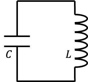
▲ A basic \(LC\) oscillator circuit contains an inductor \(L\) and a capacitor \(C\). Define the charge on the capacitor as \(Q\); a changing capacitor charge, \(\dot{Q}\), is the current flowing in the circuit. The energies stored in the capacitor and inductor are \[ E_C = \frac{Q^2}{2C}, \quad E_L = \frac{L\dot{Q}^2}{2}. \]. We may regard \(E_L\) as the kinetic-energy term \(T\) and \(E_C\) as the potential-energy term \(U\), and thereby define the Lagrangian \(L\): \[ \mathcal{L}(\dot{Q}, Q) = T - U = \frac{L\dot{Q}^2}{2} - \frac{Q^2}{2C}. \]
From the Euler–Lagrange equation, \[ \frac{d}{dt} \frac{\partial \mathcal{L}}{\partial \dot{Q}} - \frac{\partial \mathcal{L}}{\partial Q} = 0, \], we obtain \[ L\ddot{Q} + \frac{Q}{C} = 0 \implies \ddot{Q} + \frac{Q}{LC} = 0, \], which describes simple harmonic motion at frequency \(\omega = \frac{1}{\sqrt{LC}}\).
Quantizing a Classical LC Circuit
What Is Canonical Quantization?
Canonical quantization is a method for introducing quantum structure into a classical system. Its central step is to replace the Poisson structure of Hamiltonian mechanics with commutation relations. The preceding section gave the Lagrangian; a Legendre transform now yields the Hamiltonian.
LC Circuit
Basic Relations for an LC Circuit
An LC circuit consists of a capacitor \(C\) and an inductor \(L\). Their defining relations are \[ \left\{ \begin{aligned} \text{Capacitor:}\qquad I_C &= C\frac{dV_C}{dt},\\[6pt] \text{Inductor:}\qquad V_L &= L\frac{dI_L}{dt}. \end{aligned} \right. \]. Because the instantaneous power is \(IV\), the energy stored in the circuit elements can be written as \[ E=\int_{0}^{t}IV\,dt. \].
Let \(Q\) denote the charge on the capacitor, so the circuit current is \(I=\dot{Q}\). The energies stored in the capacitor and inductor are \[ \left\{ \begin{aligned} E_C &= \frac{Q^2}{2C},\\[6pt] E_L &= \frac{L\dot{Q}^{\,2}}{2}. \end{aligned} \right. \]. These forms correspond to a mass–spring system, \[ \left\{ \begin{aligned} E_C &= \frac{Q^2}{2C},\\[6pt] E_L &= \frac{L\dot{Q}^{\,2}}{2} \end{aligned} \right. \quad\longleftrightarrow\quad \left\{ \begin{aligned} V &= \frac{1}{2}Kx^2,\\[6pt] T &= \frac{1}{2}m\dot{x}^{\,2}. \end{aligned} \right. \], where \(x\) is the displacement of mass \(m\) and \(K\) is the spring constant. The mapping between the two systems is \[ Q\longleftrightarrow x, \qquad L\longleftrightarrow m, \qquad \frac{1}{C}\longleftrightarrow K. \].
Define the flux variable \(\Phi\) across the inductor: \[ \Phi \equiv \int_{0}^{t}V_L\,dt = \int_{0}^{t} L\frac{dI_L}{dt}\,dt = LI_L = L\dot{Q}. \]. Because the capacitor and inductor in the LC circuit have the same terminal voltage, \(V_L=V_C\), it follows that \[ \frac{d\Phi}{dt} = V_L = V_C = \frac{Q}{C}. \]. The relation between charge \(Q\) and flux variable \(\Phi\) is therefore \[ Q=C\dot{\Phi}. \].
Substituting \(Q=C\dot{\Phi}\) and \(\Phi=L\dot{Q}\) into the energy expression gives \[ \left\{ \begin{aligned} E_C &= \frac{Q^2}{2C} = \frac{C\dot{\Phi}^{\,2}}{2},\\[8pt] E_L &= \frac{L\dot{Q}^{\,2}}{2} = \frac{\Phi^2}{2L}. \end{aligned} \right. \]. Thus, when \(\Phi\) is used as the generalized coordinate, the capacitive energy plays the role of kinetic energy and the inductive energy plays the role of potential energy.
The LC-circuit Lagrangian \(\mathcal{L}\) is \[ \mathcal{L} = E_C-E_L = \frac{C\dot{\Phi}^{\,2}}{2} - \frac{\Phi^2}{2L}. \].
The canonical momentum \(\Pi\) corresponding to generalized coordinate \(\Phi\) is defined by \[ \Pi \equiv \frac{\partial\mathcal{L}} {\partial\dot{\Phi}} = C\dot{\Phi} = Q. \]. In an LC circuit, the canonical momentum conjugate to flux \(\Phi\) is therefore charge \(Q\).
The Hamiltonian \(\mathcal{H}\) is defined by the Legendre transform \[ \mathcal{H} \equiv \Pi\dot{\Phi}-\mathcal{L}. \]. Substituting \(\Pi=Q=C\dot{\Phi}\) gives \[ \mathcal{H} = \frac{Q^2}{2C} + \frac{\Phi^2}{2L}. \].
\[ [\hat{\Phi},\hat{Q}] = i\hbar \quad\longleftrightarrow\quad [x,p] = i\hbar. \]
Choice of Canonical Coordinate (Optional)
The canonical momentum \(\Phi_\#\) is defined by \[ \Phi_\# \equiv \frac{\partial \mathcal{L}}{\partial \dot{Q}} = \mathcal{L}\dot{Q} \leftrightarrow \dot{Q} = \frac{\Phi_\#}{L}. \]. Here \(\Phi_\#\) has the units of flux and can be regarded as the flux inside the inductor. The Hamiltonian \(H(\Phi_\#, Q)\) is defined as \[ \mathcal{H} \equiv \Phi_\# \dot{Q} - \mathcal{L} = \frac{\Phi_\#^2}{2L} + \frac{Q^2}{2C}. \].
In a quantum system, canonical coordinate \(q\) and canonical momentum \(p\) obey the commutation relation \[ [x, p] = i\hbar. \]. For the parameters used here, the quantization condition is \[ [Q, \Phi_\#] = i\hbar. \].
We currently use the notation \(\Phi_\#\), the reverse of the convention in traditional treatments. Because the Hamiltonian is symmetric in the roles of \(\Phi_\#\) and \(Q\), it can appear that either may be chosen as coordinate or momentum, even though kinetic and potential energy enter the Lagrangian asymmetrically. We therefore reverse the usual convention here, treating the flux part as the generalized coordinate \(\Phi\) and \(Q\) as the generalized momentum.
With this choice, the quantization condition becomes \[ [\Phi, Q] = i\hbar, \], which differs from our earlier choice by a minus sign: \[ \Phi = -\Phi_\#. \]. This sign can also be explained by the antisymmetry of the Lagrangian transformation.
One common explanation is that the linear inductor will later be replaced by a nonlinear inductive element, the Josephson junction, whose nonlinear term is easier to interpret as potential energy. Yet a qubit is later driven by applying a voltage to its capacitor, which would then appear to drive the kinetic rather than potential energy. For calculation, the assignment of “kinetic” and “potential” makes no physical difference.
Introduce the new variables \(a\) and \(a^\dagger\): \[ a = \sqrt{\frac{1}{2\hbar} \sqrt{\frac{L}{C}}} \left( Q + i\sqrt{\frac{C}{L}} \Phi_\# \right), \quad a^\dagger = \sqrt{\frac{1}{2\hbar} \sqrt{\frac{L}{C}}} \left( Q - i\sqrt{\frac{C}{L}} \Phi_\# \right). \]. Conversely, \[ Q = \sqrt{\frac{\hbar}{2} \sqrt{\frac{C}{L}}} (a^\dagger + a), \quad \Phi_\# = i\sqrt{\frac{\hbar}{2} \sqrt{\frac{L}{C}}} (a^\dagger - a). \].
It is straightforward to show \([a, a^\dagger] = 1\): \[ [a, a^\dagger] = aa^\dagger - a^\dagger a = \frac{1}{2\hbar} \sqrt{\frac{L}{C}} \left[ Q, \Phi_\# \right] = 1. \]. Using \(a\) and \(a^\dagger\), rewrite the Hamiltonian \(H(\Phi_\#, Q)\) as \[ \mathcal{H} = \frac{\Phi_\#^2}{2L} + \frac{Q^2}{2C} = \frac{\hbar \omega}{4} \left[ - (a^\dagger - a)^2 + (a^\dagger + a)^2 \right], \], where \(\omega = \frac{1}{\sqrt{LC}}\). Expanding gives \[ \mathcal{H} = \frac{\hbar \omega}{2} \left[ a^\dagger a + a^\dagger a + 1 \right] = \hbar \omega \left[ a^\dagger a + \frac{1}{2} \right]. \].
The final quantized Hamiltonian has adjacent energy levels separated by \(\hbar \omega\).
Interchanging the Kinetic- and Potential-Energy Terms
Strict Definition of Canonical Coordinates
To quantize correctly through commutation relations, the correspondence involving \(x, p\) must be defined strictly; otherwise a sign discrepancy can arise. From the preceding section, \[ \dot{\Phi}_\# = \frac{d}{dt} \frac{\partial \mathcal{L}}{\partial \dot{Q}} = \frac{\partial \mathcal{L}}{\partial Q} = -\frac{Q}{C} \implies Q = -C\dot{\Phi}_\#. \]. We now transform the Lagrangian \(L\) into momentum space.
Define the new Lagrangian \(\bar{\mathcal{L}}\) by \[ \bar{\mathcal{L}} \equiv \mathcal{L} - \frac{d}{dt} (\Phi_\# Q) = \mathcal{L} - \dot{\Phi}_\# Q - \Phi_\# \dot{Q}, \]. Expanding gives \[ \bar{\mathcal{L}} = \frac{L\dot{Q}^2}{2} - \frac{Q^2}{2C} - \dot{\Phi}_\# Q - \Phi_\# \dot{Q} = \frac{\Phi_\#^2}{2L} - \frac{C\dot{\Phi}_\#^2}{2} + C\dot{\Phi}_\#^2 - \frac{\Phi_\#^2}{L}, \], which simplifies to \[ \bar{\mathcal{L}} = \frac{C\dot{\Phi}_\#^2}{2} - \frac{\Phi_\#^2}{2L}. \].
Notice that now \(\mathcal{L}(Q, \dot{Q}) \to \bar{\mathcal{L}}(\Phi_\#, \dot{\Phi}_\#)\), so the roles of kinetic and potential energy are interchanged. At the same time, \(\bar{\mathcal{L}} = -\mathcal{L}\), reflecting the antisymmetry of the Lagrangian transformation. To absorb this antisymmetry, define the new variable \[ \Phi = -\Phi_\#. \], which gives \[ \bar{\mathcal{L}}(\dot{\Phi}, \Phi) = \frac{C\dot{\Phi}^2}{2} - \frac{\Phi^2}{2L}. \].
The corresponding canonical momentum \(\Pi\), using the preceding result and its relation to \(Q\), is \[ \Pi \equiv \frac{\partial \bar{\mathcal{L}}}{\partial \dot{\Phi}} = C\dot{\Phi} = -C\dot{\Phi}_\# = Q \implies \dot{\Phi} = \frac{\Pi}{C} = \frac{Q}{C}. \].
The Hamiltonian \(\bar{\mathcal{H}}\) is defined by \[ \bar{\mathcal{H}} = \Pi\dot{\Phi} - \bar{\mathcal{L}} = \frac{\Pi^2}{C} - \frac{\Pi^2}{2C} + \frac{\Phi^2}{2L} = \frac{\Pi^2}{2C} + \frac{\Phi^2}{2L}, \] and is identical to the earlier \(\mathcal{H}\). The quantization condition is now \[ [\Phi, \Pi] = [\Phi, Q] = i\hbar, \], the conventional condition.
Define new variables \(a\) and \(a^\dagger\): \[ a = \sqrt{\frac{1}{2\hbar} \sqrt{\frac{L}{C}}} \left( \sqrt{\frac{C}{L}} \Phi + iQ \right), \quad a^\dagger = \sqrt{\frac{1}{2\hbar} \sqrt{\frac{L}{C}}} \left( \sqrt{\frac{C}{L}} \Phi - iQ \right). \] Conversely: \[ \Phi = \sqrt{\frac{\hbar}{2} \sqrt{\frac{L}{C}}} (a^\dagger + a), \quad Q = i\sqrt{\frac{\hbar}{2} \sqrt{\frac{C}{L}}} (a^\dagger - a). \]
It is straightforward to show that \([a, a^\dagger] = 1\): \[ [a, a^\dagger] = aa^\dagger - a^\dagger a = \frac{1}{2\hbar} \sqrt{\frac{L}{C}} \left[ \Phi, Q \right] = 1. \] The Hamiltonian \(H(\Phi, Q)\) can therefore be rewritten as: \[ \mathcal{H} = \frac{\Phi^2}{2L} + \frac{Q^2}{2C} = \frac{\hbar}{4\sqrt{LC}} \left[ (a^\dagger + a)^2 - (a^\dagger - a)^2 \right]. \] Since \(\omega = \frac{1}{\sqrt{LC}}\), expanding gives: \[ \mathcal{H} = \frac{\hbar \omega}{4} \left[ (a^\dagger + a)^2 - (a^\dagger - a)^2 \right] = \hbar \omega \left[ a^\dagger a + \frac{1}{2} \right]. \]
Finally, we again obtain the quantized Hamiltonian, in which adjacent energy levels differ by \(\hbar \omega\).
Formal interchange of Lagrangian kinetic and potential terms
Streamlined derivation
Starting from \(L(\dot{Q}, Q)\), and using the antisymmetry between the Lagrangian kinetic and potential terms, we define the canonical momentum \(\Phi\) associated with \(\dot{Q}\) by manually inserting a minus sign to absorb that antisymmetry (otherwise the resulting Hamiltonian would be negative): \[ \Phi \equiv -\frac{\partial \mathcal{L}}{\partial \dot{Q}} \implies \dot{\Phi} = -\frac{\partial \mathcal{L}}{\partial Q}. \] We then transform the Lagrangian into \((\dot{\Phi}, \Phi)\) space—that is, the momentum-space Lagrangian \(\bar{\mathcal{L}}\): \[ \bar{\mathcal{L}} \equiv \mathcal{L} + \frac{d}{dt} (\Phi Q) = \mathcal{L} + \dot{\Phi} Q + \Phi \dot{Q}. \]
Using differentials, one can show that \(\bar{\mathcal{L}} = \bar{\mathcal{L}}(\dot{\Phi}, \Phi)\) is a function in \((\dot{\Phi}, \Phi)\) space: \[ d\bar{\mathcal{L}} = d\mathcal{L} + d(\dot{\Phi} Q) + d(\Phi \dot{Q}) = \frac{\partial \mathcal{L}}{\partial \dot{Q}} d\dot{Q} + \frac{\partial \mathcal{L}}{\partial Q} dQ + Qd\dot{\Phi} + \dot{\Phi}dQ + \dot{Q}d\Phi + \Phi d\dot{Q}. \] After expansion, because \(-\Phi = \frac{\partial \mathcal{L}}{\partial \dot{Q}}\), we obtain: \[ d\bar{\mathcal{L}} = -\Phi d\dot{Q} - \dot{\Phi} dQ + Q d\dot{\Phi} + \dot{\Phi} dQ + \dot{Q} d\Phi + \Phi d\dot{Q} = Q d\dot{\Phi} + \dot{Q} d\Phi. \]
At this point, the canonical momentum \(\Pi\) associated with \(\dot{\Phi}\) is: \[ \Pi = \frac{\partial \bar{\mathcal{L}}}{\partial \dot{\Phi}} = Q, \] which is identical to the original \(Q\). The corresponding Hamiltonian \(\bar{\mathcal{H}}\) is defined as: \[ \bar{\mathcal{H}} = \Pi \dot{\Phi} - \bar{\mathcal{L}} = Q\dot{\Phi} - \mathcal{L} - \dot{\Phi} Q - \Phi \dot{Q} = -\mathcal{L} - \Phi \dot{Q}. \] Its final form is: \[ \bar{\mathcal{H}}(Q, \Phi) = -\mathcal{L} - \Phi \dot{Q}. \]
This lets us streamline the subsequent derivations by following only these steps:
- Write down \(L(\dot{Q}, Q)\).
- Define \(\Phi \equiv -\frac{\partial \mathcal{L}}{\partial \dot{Q}}\) and obtain the relation among \(\dot{Q}\) and \(\Phi\).
- Directly find the corresponding Hamiltonian: \[ \bar{\mathcal{H}}(Q, \Phi) = -\mathcal{L} - \Phi \dot{Q}, \] and substitute \(\dot{Q}\) into the relation above.
- Quantization condition: \[ [Q, \Phi] = i\hbar. \]
This avoids the cumbersome transformation \(L(\dot{Q}, Q) \to \bar{\mathcal{L}}(\dot{\Phi}, \Phi) \to \bar{\mathcal{H}}(Q, \Phi)\). This is especially useful when external-force coupling terms are introduced later—for example, when deriving how a qubit is driven and read out, how an external signal interacts with a qubit, or how two qubits couple. The longer derivation would produce a situation analogous to momentum \(p \to p - eA\) in an electromagnetic field, making the intermediate transformations extremely complicated.
Note: Observe that: \[ \bar{\mathcal{H}}(Q, \Phi) = -\mathcal{L} - \Phi \dot{Q} = -\mathcal{L} + \frac{\partial \mathcal{L}}{\partial \dot{Q}} \dot{Q} = H(\Phi, Q). \] \(H(\Phi, Q)\) is the familiar conventional Hamiltonian. At the same time, \(\bar{\mathcal{H}} = H\) once again reveals the symmetry between the kinetic and potential terms of the Hamiltonian.
Advanced throughline: Circuit → Lagrangian → Hamiltonian → Spectrum
(W2-C1, W2-D1, W2-D2)For node flux \(\Phi\), the capacitive network provides the kinetic term, while inductors and Josephson junctions provide the potential term:
\[\mathcal L=\frac12\dot{\Phi}^{T} C\dot{\Phi}-U(\Phi),\qquad Q=\frac{\partial\mathcal L}{\partial\dot{\Phi}}\]
A Legendre transform gives \(H(\Phi, Q)\), after which we impose \([\hat\Phi_i,\hat Q_j]=i\hbar\delta_{ij}\). A linear LC circuit produces only equally spaced energy levels; it is the Josephson term
\[U_J(\varphi)=-E_J\cos\varphi,\qquad E_J=\frac{\Phi_0 I_c}{2\pi}\]
that breaks harmonicity and allows selective control of the two lowest levels. In an advanced course, students need to complete the full path from schematic to Hamiltonian at least once; memorizing the transmon formula is not enough to predict the consequences of parasitic modes, coupling, or layout changes.
Boundary:This week does not go deeply into the microscopic BCS derivation. Here, superconductors primarily provide a macroscopic phase, low-loss wiring, and the Josephson element. Microscopic material loss is deferred to T6.
Classroom Integration and Assessment
Discussion question: For a single-node circuit containing \(C\), \(L\), and a JJ, write down \(\mathcal L\), the canonical charge, and \(H\); then identify which parameter is controlled by layout or fabrication.
Completion criterion: Students must leave a checkable derivation, relationship diagram, comparison table, or architecture decision, and must be able to explain its physical assumptions and engineering costs.
Core and Further Reading
- Introduction to Quantum Electromagnetic CircuitsU. Vool and M. H. Devoret, International Journal of Circuit Theory and Applications 45, 897–934 (2017).A core reading on going from a circuit diagram and Lagrangian to a quantum Hamiltonian.
- Black-box Superconducting Circuit QuantizationS. E. Nigg et al., Physical Review Letters 108, 240502 (2012).Turns a distributed electromagnetic environment and Josephson nonlinearity into an effective Hamiltonian.
- A Quantum Engineer's Guide to Superconducting QubitsP. Krantz et al., Applied Physics Reviews 6, 021318 (2019).A foundational review of control, coherence, readout, and engineering parameters.
- Engineering High-Coherence Superconducting QubitsI. Siddiqi, Nature Reviews Materials 6, 875–891 (2021).Design trade-offs among different qubit architectures, material loss, and coherence.
Question 3: Why is the simplest artificial atom still not a qubit?
A quantized LC circuit already has discrete energy levels:
\[ \hat H_{LC}=\frac{\hat Q^2}{2C}+\frac{\hat\Phi^2}{2L} =\hbar\omega\left(\hat a^\dagger\hat a+\frac12\right), \qquad \omega=\frac1{\sqrt{LC}}. \]
First establish that an LC circuit really is a quantum system
Define the characteristic impedance \(Z=\sqrt{L/C}\), so the flux and charge operators can be written as
\[ \hat\Phi=\Phi_{\rm zpf}(\hat a+\hat a^\dagger), \qquad \hat Q=-iQ_{\rm zpf}(\hat a-\hat a^\dagger), \]
\[ \Phi_{\rm zpf}=\sqrt{\frac{\hbar Z}{2}}, \qquad Q_{\rm zpf}=\sqrt{\frac{\hbar}{2Z}}, \qquad \Phi_{\rm zpf}Q_{\rm zpf}=\frac{\hbar}{2}. \]
Even in the ground state, flux and charge retain zero-point fluctuations. The energy eigenstates \(\ket m\) are also genuinely discrete:
\[ E_m=\hbar\omega\left(m+\frac12\right), \qquad m=0,1,2,\ldots \]
The problem, then, is not that the LC oscillator is “insufficiently quantum.” Quite the opposite: it is an overly ideal linear quantum system in which every rung obeys exactly the same rule.
An equally spaced spectrum makes all adjacent transition frequencies coincide
The transition frequency between adjacent levels is
\[ \omega_{m,m+1} =\frac{E_{m+1}-E_m}{\hbar} =\omega, \]
Therefore,
\[ \omega_{01}=\omega_{12}=\omega_{23}=\cdots. \]
A resonant microwave tone sees not only \(\ket0\leftrightarrow\ket1\) but also every higher transition. Frequency selectivity cannot tell the system to use only the two lowest levels.
The drive Hamiltonian shows why leakage is unavoidable
Suppose the oscillator is driven by a capacitively coupled microwave voltage. Ignoring a coupling prefactor that does not affect the main point, the control term can be written as
\[ \hat H_d(t) =\hbar\epsilon(t)(\hat a+\hat a^\dagger). \]
The matrix element between adjacent levels is
\[ \langle m+1|\hat a+\hat a^\dagger|m\rangle =\sqrt{m+1}. \]
The drive initially pushes \(\ket0\) toward \(\ket1\). Once \(\ket1\) acquires population, the same frequency also drives \(\ket1\rightarrow\ket2\) exactly on resonance, with a matrix element larger by a factor of \(\sqrt2\). The same pattern continues upward. Therefore, \(\{\ket0,\ket1\}\) is not a closed invariant subspace under this control.
A stronger statement: a linear drive creates a coherent state, not a pure \(\ket1\) state
Under the rotating-wave approximation, a driven harmonic oscillator can be written as
\[ \hat H_{\rm rot}(t) =\hbar\bigl[\epsilon(t)\hat a^\dagger+\epsilon^*(t)\hat a\bigr]. \]
If the initial state is the vacuum, any such linear pulse can only produce a displacement:
\[ \ket0\longrightarrow\hat D(\alpha)\ket0=\ket\alpha, \qquad P_m=e^{-|\alpha|^2}\frac{|\alpha|^{2m}}{m!}. \]
To maximize \(P_1\) one must choose \(|\alpha|^2=1\), but then \(P_1^{\rm max}=e^{-1}\approx0.368\), and the remaining population is still distributed over \(\ket0,\ket2,\ldots\). In other words, applying a conventional qubit “\(\pi\) pulse” to a bare harmonic oscillator cannot deterministically flip \(\ket0\) to \(\ket1\).
A qubit also requires spectral addressability
Define the anharmonicity
\[ \alpha\equiv\omega_{12}-\omega_{01}. \]
For a harmonic oscillator, \(\alpha=0\). Only when nonlinearity makes \(\alpha\neq0\) can the drive frequency select the computational transition through \(\omega_{01}\) while remaining off-resonant from \(\omega_{12}\). For a simple pulse, we generally want
\[ |\alpha|\gg\Omega_R,\;\kappa,\;\gamma_\phi, \]
where \(\Omega_R\) is the Rabi rate. A faster drive has a broader bandwidth, and the leakage amplitude typically increases on the scale of \(\Omega_R/|\alpha|\); a slower drive instead accumulates more decoherence. This is the speed–leakage trade-off later addressed by pulse shaping and DRAG control.
A precise statement: A harmonic oscillator is not incapable of carrying quantum information. With multiple Fock states, cat states, or another bosonic encoding, an oscillator can still serve as a logical qubit. But if only ordinary linear microwave control is allowed, a bare LC oscillator does not naturally provide an independently controllable two-lowest-level qubit.
In-class task: Draw harmonic and anharmonic spectra and mark which transitions are connected by a drive at the same frequency.
Conclusion to Question 3:“Discrete energy levels” only guarantee that the system is quantum; “unequally spaced energy levels” are what make \(\ket0\leftrightarrow\ket1\) frequency-selective and suppress leakage to a controllable level.
2.2 Why Nonlinearity Is Necessary
If a quantum circuit has equally spaced levels, the frequency from \(\ket{0}\) to \(\ket{1}\) is identical to the frequency from \(\ket{1}\) to \(\ket{2}\). Microwave control therefore cannot address only the qubit subspace \(\ket{0}, \ket{1}\) and will readily excite higher levels.
A Josephson junction supplies the nonlinear inductance required by superconducting quantum circuits. Through this nonlinearity, a superconducting circuit can acquire unequally spaced energy levels, allowing its two lowest levels to serve as a qubit.
4.1 From LC Circuit to Quantum LC Oscillator
In a classical circuit, an LC oscillator exchanges energy between its capacitor and inductor. The capacitor stores electric-field energy, while the inductor stores magnetic-field energy. Quantizing the LC oscillator gives equally spaced energy levels:
\[ E_m = \hbar\omega\left(m + \frac{1}{2}\right) \]
Such a harmonic oscillator is unsuitable as a qubit because adjacent levels have the same spacing, so a control pulse cannot select only the \(\ket{0} \leftrightarrow \ket{1}\) transition.
Question 4: How does a Josephson junction shape the energy levels of an artificial atom?
Josephson tunneling provides a nondissipative, phase-controlled nonlinear element:
\[ I=I_c\sin\varphi, \qquad V=\frac{\Phi_0}{2\pi}\dot\varphi, \qquad U_J(\varphi)=-E_J\cos\varphi. \]
The Josephson energy is not a separate assumption: it follows by integrating the two Josephson relations
The supercurrent branch of an ideal junction obeys \(I=I_c\sin\varphi\), while the phase evolves with voltage according to \(V=(\Phi_0/2\pi)\dot\varphi\). The instantaneous power flowing into the element is
\[ P=IV =I_c\sin\varphi\, \frac{\Phi_0}{2\pi}\dot\varphi. \]
If this power is stored in the junction potential, then
\[ \frac{dU_J}{dt} =\frac{dU_J}{d\varphi}\dot\varphi =\frac{\Phi_0 I_c}{2\pi}\sin\varphi\,\dot\varphi. \]
and therefore
\[ \frac{dU_J}{d\varphi}=E_J\sin\varphi, \qquad E_J\equiv\frac{\Phi_0 I_c}{2\pi} =\frac{\hbar I_c}{2e}, \]
Integrating gives
\[ U_J(\varphi)=-E_J\cos\varphi+\text{constant}. \]
Thus, saying that “a Josephson junction provides a cosine potential” does not mean forcing the circuit into a preconceived atomic model. The energy landscape follows directly from the measurable current–phase relation.
It behaves like an inductor, but not a linear one
For a linear inductor, \(I=\Phi/L\), so the potential is always quadratic. For a junction, \(\dot I=I_c\cos\varphi\,\dot\varphi\). Comparing \(V=L_J\dot I\) gives the differential inductance
\[ L_J(\varphi) =\frac{\Phi_0}{2\pi I_c\cos\varphi}. \]
\(L_J\) varies with phase: this is the circuit-language description of nonlinearity. For small amplitudes with \(\varphi\approx0\), \(L_J(0)=\Phi_0/(2\pi I_c)\) and the junction appears approximately linear; at larger amplitudes, the variation of \(\cos\varphi\) can no longer be neglected. At the same time, the ideal Josephson supercurrent is nondissipative, so a junction can provide strong nonlinearity in a low-loss circuit—a combination difficult to achieve with an ordinary resistor or semiconductor diode. Real devices still have junction capacitance, quasiparticle loss, and material defects; “ideally nondissipative” must not be mistaken for completely lossless.
With capacitance included, phase becomes a quantum coordinate moving in a cosine potential
Combine the junction with a total capacitance \(C_\Sigma\) and define the charging energy as
\[ E_C\equiv\frac{e^2}{2C_\Sigma}. \]
The Hamiltonian becomes
\[ \hat H =4E_C(\hat n-n_g)^2-E_J\cos\hat\varphi. \]
In the “quantum particle” picture, \(\varphi\) is position and \(n\) is momentum; \(E_C\) sets the kinetic-energy scale, while \(E_J\) sets the depth of the periodic potential. Changing the junction critical current changes \(E_J\), and changing the shunt capacitance changes \(E_C\). The “mass, confinement strength, and spectrum” of this artificial atom can therefore all be designed through its circuit.
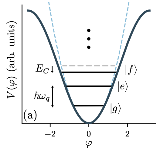
Higher-order terms of the cosine break equal spacing
In the linearized approximation, retain only the quadratic term near a potential minimum:
\[ -E_J\cos\varphi =-E_J+\frac{E_J}{2}\varphi^2 -\frac{E_J}{24}\varphi^4 +\frac{E_J}{720}\varphi^6-\cdots. \]
The quadratic potential of a linear inductor can produce only a harmonic spectrum; the cosine potential of a Josephson junction provides a nonlinear inductance. When the cosine is expanded, the quadratic term establishes the dominant oscillation frequency, while the higher-order terms break the equal spacing and produce an anharmonic spectrum that can be selectively controlled.
First treat the quadratic part as a harmonic oscillator:
\[ \hat H_0 =4E_C\hat n^2+\frac{E_J}{2}\hat\varphi^2-E_J, \qquad \hbar\omega_p=\sqrt{8E_JE_C}. \]
The corresponding zero-point amplitudes may be chosen as
\[ \hat\varphi=\varphi_{\rm zpf}(\hat a+\hat a^\dagger), \qquad \hat n=i n_{\rm zpf}(\hat a^\dagger-\hat a), \]
\[ \varphi_{\rm zpf} =\left(\frac{2E_C}{E_J}\right)^{1/4}, \qquad n_{\rm zpf} =\left(\frac{E_J}{32E_C}\right)^{1/4}, \qquad \varphi_{\rm zpf}n_{\rm zpf}=\frac12. \]
Now treat the quartic term \(-E_J\hat\varphi^4/24\) as a first-order perturbation. Because
\[ \langle m|(\hat a+\hat a^\dagger)^4|m\rangle =6m^2+6m+3, \]
we obtain the low-energy approximation
\[ E_m\approx -E_J+\sqrt{8E_JE_C}\left(m+\frac12\right) -\frac{E_C}{12}(6m^2+6m+3). \]
Thus adjacent transitions no longer have the same frequency:
\[ \hbar\omega_{m,m+1} \approx\sqrt{8E_JE_C}-E_C(m+1), \]
\[ \hbar\omega_{01}\approx\sqrt{8E_JE_C}-E_C, \qquad \hbar\omega_{12}\approx\sqrt{8E_JE_C}-2E_C, \]
\[ \alpha\equiv\omega_{12}-\omega_{01} \approx-\frac{E_C}{\hbar}. \]
The minus sign means that the spacing between adjacent levels decreases at higher energy. This result comes from the negative quartic correction of the cosine; it is precisely what detunes the \(\omega_{01}\) drive from \(\omega_{12}\) and makes selective control of the two lowest levels possible.
The same cosine provides two complementary intuitions in two different bases
- phase basis: \(-E_J\cos\varphi\) forms periodic wells; as \(E_J/E_C\) increases, the low-energy wavefunction becomes more localized near one minimum.
- charge basis: \(-E_J\cos\hat\varphi\) couples \(\ket n\) and \(\ket{n\pm1}\), turning crossings of the bare charge-state energies into avoided crossings.
Conclusion to Question 4: A Josephson junction does not simply “add another inductor”; it replaces a quadratic potential with a cosine potential designable through \(E_J\). Its quadratic part sets the dominant frequency, while its quartic and higher-order terms create anharmonicity. This is how an artificial atom acquires a controllable spectrum.
3.3 Josephson Junction
A Josephson junction consists of two superconductors separated by an ultrathin insulating layer. It is commonly called an SIS junction: superconductor–insulator–superconductor. Although the middle layer is insulating, Cooper pairs can still cross the junction by quantum tunneling and form a Josephson current.
Josephson Relations
The current through a Josephson junction depends nonlinearly on the phase difference:
\[ I = I_c \sin\varphi \]
When a voltage \(V\) exists across the junction, the phase difference evolves in time:
\[ V = \frac{\Phi_0}{2\pi}\frac{d\varphi}{dt} \]
where \(\Phi_0 = h/2e\) is the superconducting flux quantum. The Josephson energy can be written as:
\[ E_J = \frac{\Phi_0 I_c}{2\pi} \]
3.4 Josephson Junction as a Nonlinear Inductor
The key value of a Josephson junction is that it provides nonlinear inductance. The energy of an ordinary linear inductor is approximately quadratic in phase; the Josephson-junction energy is instead:
\[ U_J(\varphi) = -E_J \cos\varphi \]
This cosine potential makes the circuit's energy levels unequally spaced, allowing the two lowest levels of the quantum oscillator to be selected as a qubit.
Core concept
Without a Josephson junction, a superconducting LC circuit is only an approximate harmonic oscillator. With a Josephson junction, the circuit gains enough nonlinearity to form an addressable quantum two-level system.
Learning Check
- Why can Cooper pairs cross the insulating layer of a Josephson junction?
- What is the relation between Josephson current and phase difference?
- Why can a Josephson junction be regarded as a nonlinear inductor?
The nonlinear inductive nature of the Josephson junction
Nonlinearity enables precise qubit control
Quantum description of a Josephson junction
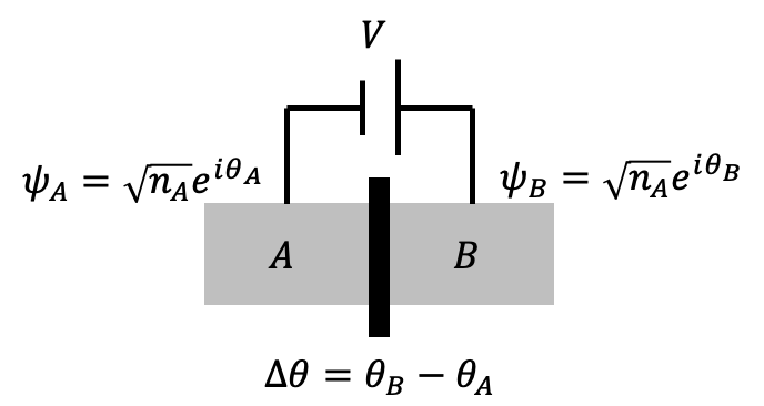
▲ A Josephson junction whose intrinsic material properties are described by \(H_0\). A voltage \(V\) is applied across the junction, and the interaction between the superconducting wavefunctions is represented by \(K\), with equation of motion: \[ i\hbar \frac{\partial}{\partial t} \begin{pmatrix} \sqrt{n_A} e^{i\theta_A} \\ \sqrt{n_B} e^{i\theta_B} \end{pmatrix} = \begin{pmatrix} H_0 - \frac{qV}{2} & K \\ K & H_0 + \frac{qV}{2} \end{pmatrix} \begin{pmatrix} \sqrt{n_A} e^{i\theta_A} \\ \sqrt{n_B} e^{i\theta_B} \end{pmatrix}. \] For \(q = -2e\) (a Cooper pair), the equation becomes: \[ i\hbar \frac{\partial}{\partial t} \begin{pmatrix} \sqrt{n_A} e^{i\theta_A} \\ \sqrt{n_B} e^{i\theta_B} \end{pmatrix} = \begin{pmatrix} H_0 + eV & K \\ K & H_0 - eV \end{pmatrix} \begin{pmatrix} \sqrt{n_A} e^{i\theta_A} \\ \sqrt{n_B} e^{i\theta_B} \end{pmatrix}. \]
Complete derivation of \(\theta_A, n_A \)
The first equation is: \[ i\hbar \frac{\partial}{\partial t} (\sqrt{n_A} e^{i\theta_A}) = \frac{i}{2} \frac{e^{i\theta_A}}{\sqrt{n_A}} \frac{\partial n_A}{\partial t} - \sqrt{n_A} e^{i\theta_A} \frac{\partial \theta_A}{\partial t} = (H_0 + eV) \sqrt{n_A} e^{i\theta_A} + K\sqrt{n_B} e^{i\theta_B}. \] Separating real and imaginary parts gives: \[ \frac{i}{2}\hbar \frac{\partial n_A}{\partial t} - n_A \hbar \frac{\partial \theta_A}{\partial t} = (H_0 + eV)n_A + K\sqrt{n_A n_B} e^{i(\theta_B - \theta_A)}. \] Its complex-conjugate equation is: \[ -\frac{i}{2}\hbar \frac{\partial n_A}{\partial t} - n_A \hbar \frac{\partial \theta_A}{\partial t} = (H_0 + eV)n_A + K\sqrt{n_A n_B} e^{-i(\theta_B - \theta_A)}. \]
| Adding the two equations gives: \[ -2n_A \hbar \frac{\partial \theta_A}{\partial t} = 2(H_0 + eV)n_A + 2K\sqrt{n_A n_B} \cos(\theta_B - \theta_A), \] Rearranging yields the equation for \(\theta_A\): \[ \hbar \frac{\partial \theta_A}{\partial t} = -(H_0 + eV) - K\sqrt{\frac{n_B}{n_A}} \cos(\theta_B - \theta_A). \] |
|---|
| Subtracting the two equations gives: \[ i\hbar \frac{\partial n_A}{\partial t} = 2iK\sqrt{n_A n_B} \sin(\theta_B - \theta_A), \] That is: \[ \hbar \frac{\partial n_A}{\partial t} = 2K\sqrt{n_A n_B} \sin(\theta_B - \theta_A). \] |
Complete derivation of \(\theta_B, n_B \)
The second equation is: \[ i\hbar \frac{\partial}{\partial t} (\sqrt{n_B} e^{i\theta_B}) = \frac{i}{2} \frac{e^{i\theta_B}}{\sqrt{n_B}} \frac{\partial n_B}{\partial t} - \sqrt{n_B} e^{i\theta_B} \frac{\partial \theta_B}{\partial t} = K\sqrt{n_A} e^{i\theta_A} + (H_0 - eV)\sqrt{n_B} e^{i\theta_B}. \] Splitting it gives: \[ \frac{i}{2}\hbar \frac{\partial n_B}{\partial t} - n_B \hbar \frac{\partial \theta_B}{\partial t} = K\sqrt{n_A n_B} e^{-i(\theta_B - \theta_A)} + (H_0 - eV)n_B. \] Its complex-conjugate equation is: \[ -\frac{i}{2}\hbar \frac{\partial n_B}{\partial t} - n_B \hbar \frac{\partial \theta_B}{\partial t} = K\sqrt{n_A n_B} e^{i(\theta_B - \theta_A)} + (H_0 - eV)n_B. \]
| Adding the two equations gives: \[ -2n_B \hbar \frac{\partial \theta_B}{\partial t} = 2K\sqrt{n_A n_B} \cos(\theta_B - \theta_A) + 2(H_0 - eV)n_B, \] Rearranging yields the equation for \(\theta_B\): \[ \hbar \frac{\partial \theta_B}{\partial t} = -(H_0 - eV) - K\sqrt{\frac{n_A}{n_B}} \cos(\theta_B - \theta_A). \] |
|---|
| Subtracting the two equations gives: \[ i\hbar \frac{\partial n_B}{\partial t} = -2iK\sqrt{n_A n_B} \sin(\theta_B - \theta_A), \] That is: \[ \hbar \frac{\partial n_B}{\partial t} = -2K\sqrt{n_A n_B} \sin(\theta_B - \theta_A). \] |
Rearrangement gives the following equations:
- For \(\theta_A\): \[ \hbar \frac{\partial \theta_A}{\partial t} = -(H_0 + eV) - K\sqrt{\frac{n_B}{n_A}} \cos(\theta_B - \theta_A). \]
- For \(\theta_B\): \[ \hbar \frac{\partial \theta_B}{\partial t} = -(H_0 - eV) - K\sqrt{\frac{n_A}{n_B}} \cos(\theta_B - \theta_A). \]
- For \(n_A\): \[ \hbar \frac{\partial n_A}{\partial t} = 2K\sqrt{n_A n_B} \sin(\theta_B - \theta_A). \]
- For \(n_B\): \[ \hbar \frac{\partial n_B}{\partial t} = -2K\sqrt{n_A n_B} \sin(\theta_B - \theta_A). \]
Define the phase difference \(\Delta \theta = \theta_B - \theta_A\) and subtract the first two equations to obtain: \[ \hbar \frac{\partial \Delta \theta}{\partial t} = 2eV + \frac{K}{\hbar} \left( \frac{n_B - n_A}{\sqrt{n_A n_B}} \right) \cos\Delta \theta. \] Combine the latter two equations and define the current \(I\) as: \[ -\frac{\partial n_A}{\partial t} = \frac{\partial n_B}{\partial t} \equiv \frac{I}{-2e}. \] Rearranging gives: \[ I = \frac{4eK}{\hbar} \sqrt{n_A n_B} \sin\Delta \theta \equiv I_c \sin\Delta \theta, \] where \(I_c\) is the critical current of the Josephson junction.
Define the nonlinear inductance of the Josephson junction: \[ L_J(\Delta \theta) = \left(\frac{2e}{\hbar I_c \cos\Delta \theta}\right). \] The energy stored in an inductor is: \[ E = \int IV dt = \int I_0 \sin\Delta \theta \cdot \frac{\hbar}{q} \frac{\partial \Delta \theta}{\partial t} dt = -\frac{I_0 \hbar}{2e} \cos\Delta \theta \equiv -\frac{I_0 \Phi_0}{2\pi} \cos\Delta \theta, \] where the flux quantum is \(\Phi_0 = \frac{2\pi\hbar}{2e}\), and define: \[ E_J = \frac{I_0 \Phi_0}{2\pi}. \]
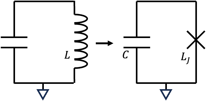
▲ A linear \(LC\) circuit becomes a nonlinear \(LC\) circuit by incorporating the nonlinear inductance of a Josephson junction. \(L_J\) is the junction inductance.
4.2 Nonlinear LC Circuit
A transmon can be understood as a nonlinear LC oscillator. It replaces an ordinary linear inductor with a Josephson junction and adds a large shunt capacitance. The Josephson junction supplies nonlinearity, while the shunt capacitor lowers the charging energy, making the qubit insensitive to offset-charge noise.
The basic transmon circuit contains:
- One Josephson junction or SQUID loop.
- A large shunt capacitor.
- Capacitive coupling to microwave control lines, a readout resonator, or a coupler.
Question 5: Why is the artificial atom ultimately designed as a transmon?
\[ \hat H_{\mathrm T}=4E_C(\hat n-n_g)^2-E_J\cos\hat\varphi. \]
A charge qubit is highly sensitive to offset charge \(n_g\). By increasing the shunt capacitance, a transmon lowers \(E_C\) and raises \(E_J/E_C\), exponentially suppressing the charge dispersion of the energy with respect to \(n_g\). The cost is a smaller magnitude of anharmonicity, requiring a new trade-off between control selectivity and gate speed.
First identify the problem with the original charge qubit
In the charge basis, first set \(E_J=0\). Each integer Cooper-pair number \(n\) then corresponds to a charging parabola:
\[ E_n(n_g)=4E_C(n-n_g)^2. \]
\(n_g\) is set by the gate voltage, background trapped charge, and environmental offset-charge fluctuations. Near \(n_g=1/2\), retaining only \(\ket{n=0}\) and \(\ket{n=1}\), Josephson tunneling gives the approximate matrix
\[ \hat H_{\{0,1\}} \approx \begin{pmatrix} 4E_Cn_g^2 & -E_J/2\\ -E_J/2 & 4E_C(1-n_g)^2 \end{pmatrix}. \]
so the two-level splitting is approximately
\[ \hbar\omega_{01} \approx\sqrt{\bigl[4E_C(1-2n_g)\bigr]^2+E_J^2}. \]
At exactly \(n_g=1/2\) there is a charge sweet spot, \(\partial\omega_{01}/\partial n_g=0\); but once the operating point drifts away, the frequency changes rapidly. If the background charge jumps, the qubit frequency jumps with it. Precise biasing at one point alone is not robust hardware protection.
The transmon's hardware move is simple: make the capacitance large
For total capacitance \(C_\Sigma\),
\[ E_C=\frac{e^2}{2C_\Sigma}. \]
Adding a large shunt capacitor increases \(C_\Sigma\) and lowers \(E_C\), while the junction critical current can still set \(E_J\) independently. Thus \(E_J/E_C\) can be shifted from the charge-qubit regime toward the transmon regime of \(E_J/E_C\gg1\). This does not introduce a different Hamiltonian; it moves the same Hamiltonian into another parameter regime.
In the phase picture, larger \(E_J/E_C\) localizes low-energy wavefunctions near a cosine minimum and reduces the quantum phase-slip amplitude between neighboring wells. Offset charge \(n_g\) plays the role of a boundary phase for the periodic potential; the dependence of energy on \(n_g\) comes precisely from interwell tunneling. As the relative barrier height grows, the energy band flattens with respect to \(n_g\).
The key is not merely that it becomes smaller: charge dispersion is exponentially suppressed
In the asymptotic regime \(E_J/E_C\gg1\), the dominant dependence of an energy level on offset charge can be written as
\[ E_m(n_g)\approx\bar E_m -\frac{\epsilon_m}{2}\cos(2\pi n_g), \]
where the leading scale of the charge-dispersion amplitude is
\[ \epsilon_m \propto E_C\, \exp\!\left[-\sqrt{8E_J/E_C}\right] \times \text{algebraic prefactor}. \]
As \(E_J/E_C\) is increased, \(\partial\omega_{01}/\partial n_g\) does not merely fall slowly as \(1/(E_J/E_C)\); it receives exponential suppression. The transmon's value lies in this asymmetric exchange: a relatively modest parameter change buys very strong suppression of charge-noise dephasing.
But the nonlinearity is not preserved for free
Question 4 gave
\[ \hbar\omega_{01}\approx\sqrt{8E_JE_C}-E_C, \qquad \alpha\equiv\omega_{12}-\omega_{01} \approx-\frac{E_C}{\hbar}. \]
The shunt capacitance lowers \(E_C\), so \(|\alpha|\) also decreases approximately linearly. Fortunately, charge dispersion is exponentially suppressed, whereas anharmonicity decreases only linearly with \(E_C\). A practical parameter window therefore exists in which charge noise is already weak but \(\omega_{01}\) and \(\omega_{12}\) remain distinguishable.
For a target transition frequency and anharmonicity, these two approximations can also be inverted for a first-pass design:
\[ \frac{E_C}{h}\approx\frac{|\alpha|}{2\pi}, \qquad \frac{E_J}{E_C} \approx\frac18 \left(\frac{hf_{01}+E_C}{E_C}\right)^2. \]
A real design still requires numerical diagonalization, a junction-fabrication model, and electromagnetic simulation. Nevertheless, these two equations already show the directional relations among pad capacitance, junction critical current, frequency, and leakage.
Protection does not turn off control along with noise
A capacitive microwave drive couples primarily through \(\hat n\). In the harmonic approximation,
\[ |\langle0|\hat n|1\rangle| \approx \left(\frac{E_J}{32E_C}\right)^{1/4}\neq0. \]
Thus, increasing \(E_J/E_C\) suppresses charge dispersion without eliminating the \(0\leftrightarrow1\) electric-dipole matrix element. The transmon therefore retains effective microwave drive and dispersive readout. The converse is that the same nonzero matrix element means a transmon is not automatically immune to all high-frequency electric noise. It primarily addresses low-frequency offset-charge dephasing, not relaxation in general.
Fixed-frequency and tunable transmons introduce the next trade-off
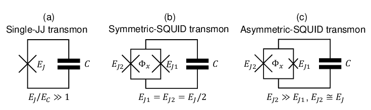
A single junction gives a fixed \(E_J\), with a simpler structure and no additional flux-noise channel; the cost is that fabrication variation directly becomes frequency spread and may cause frequency collisions. If a symmetric dc SQUID replaces the single junction, then
\[ E_{J,\mathrm{eff}}(\Phi_{\rm ext}) =2E_{J0} \left|\cos\!\left(\pi\frac{\Phi_{\rm ext}}{\Phi_0}\right)\right|, \]
The qubit frequency becomes tunable, allowing collisions to be avoided or flux-mediated gates to be performed. But away from the flux sweet spot, \(\partial\omega_{01}/\partial\Phi_{\rm ext}\neq0\); flux noise, control-line crosstalk, and calibration overhead all increase.
Reassessing the transmon with four design criteria
- Dephasing protection: \(\partial\omega_{01}/\partial n_g\) receives exponential suppression from charge dispersion.
- Relaxation protection: There is no generic \(\langle0|\hat O_{\rm noise}|1\rangle\approx0\); material loss, Purcell loss, and high-frequency electric noise must still be engineered separately.
- Controllability: \(\langle0|\hat n|1\rangle\neq0\), preserving effective microwave control and readout coupling.
- Leakage suppression: \(\Delta_{\rm leakage}\sim\hbar|\alpha|\) is finite; gate speed, pulse shaping, and residual anharmonicity must be balanced.
- Benefits: lower charge dispersion, mature microwave control, and a designable frequency range.
- Costs: weaker anharmonicity, possible leakage, and different noise and calibration burdens for fixed and tunable designs.
- Design principle: the transmon is not the “best artificial atom,” but a successful parameter choice balancing noise sensitivity, control, and manufacturability.
Conclusion for this week: Discrete energy levels alone do not make a qubit. Josephson nonlinearity must create a selectively controllable spectrum, after which \(E_J/E_C\) tunes the trade-off between charge sensitivity and anharmonicity. The transmon became mainstream not because it eliminates every source of noise, but because exponential-versus-linear scaling places it at an especially effective Pareto point that remains controllable and manufacturable.
Existing derivations and supplementary material
Properties of the transmon
The current mainstream superconducting qubit
Ref:
DOI:10.48550/arXiv.2203.04164
Unit 4: Transmon Qubit
4.3 Transmon Hamiltonian
The transmon Hamiltonian can be written as:
\[ \hat{H}_{\mathrm{transmon}} = 4E_C(\hat{n} - n_g)^2 - E_J\cos\hat{\varphi} \]
where:
- \(\hat{n}\): Cooper pair number operator.
- \(\hat{\varphi}\): the superconducting phase difference across the Josephson junction.
- \(n_g\): offset charge, representing environmental charge noise or gate-induced charge.
- \(E_C = e^2 / 2C_\Sigma\): the charging energy, set by the total capacitance \(C_\Sigma\).
- \(E_J = \Phi_0 I_c / 2\pi\): the Josephson energy, set by the junction critical current.
An important transmon design condition is:
\[ \frac{E_J}{E_C} \gg 1 \]
In this regime, the sensitivity of the energy levels to offset charge \(n_g\) is strongly suppressed, while enough anharmonicity remains for the two lowest levels to serve as a qubit.
4.4 Energy Spectrum and Anharmonicity
Under the approximation \(E_J/E_C \gg 1\), the lowest transmon levels form an approximate weakly anharmonic oscillator. Its \(\ket{0} \rightarrow \ket{1}\) transition frequency is approximately:
\[ \omega_{01} \approx \frac{\sqrt{8E_JE_C} - E_C}{\hbar} \]
The transmon anharmonicity is approximately:
\[ \alpha = \omega_{12} - \omega_{01} \approx -\frac{E_C}{\hbar} \]
Anharmonicity is an important parameter for quantum-gate control. If \(|\alpha|\) is too small, microwave pulses readily cause leakage into \(\ket{2}\); if \(|\alpha|\) is too large, it usually implies larger \(E_C\) and potentially greater charge-noise sensitivity. A transmon must therefore balance charge-noise protection against control selectivity.
4.5 Design of \(E_C\) and \(E_J\)
The core of transmon design is choosing suitable \(E_C\), \(E_J\), and \(E_J/E_C\). These parameters are set respectively by chip geometry, materials, and the Josephson-junction process.
| Parameter | Definition | Determined by | Design impact |
|---|---|---|---|
| \(E_C\) | \(e^2/2C_\Sigma\) | Total capacitance, pad area, coupling capacitance, and packaging environment | Sets anharmonicity and charge-noise sensitivity |
| \(E_J\) | \(\Phi_0 I_c/2\pi\) | Josephson-junction area, oxide thickness, and critical-current density | Sets qubit frequency and potential depth |
| \(E_J/E_C\) | Ratio of Josephson energy to charging energy | Joint design of the junction and capacitor | Controls the trade-off between charge dispersion and anharmonicity |
4.6 Fixed-Frequency and Tunable Transmon
Transmons may be divided into fixed-frequency and tunable types. A fixed-frequency transmon uses a single Josephson junction, so its frequency is largely fixed after fabrication. A tunable transmon replaces the single junction with a SQUID loop, allowing the effective Josephson energy to be controlled by an applied magnetic flux.
\[ E_J(\Phi_{\mathrm{ext}}) \approx E_{J,\mathrm{max}} \left| \cos\left(\pi\frac{\Phi_{\mathrm{ext}}}{\Phi_0}\right) \right| \]
A tunable transmon offers greater control flexibility for frequency tuning, two-qubit gates, and avoiding frequency collisions, but it also increases sensitivity to flux noise.
Design intuition
The transmon's success comes from a simple but profound design strategy: use a larger capacitance to lower \(E_C\), sacrifice some anharmonicity, and gain exponential protection against charge noise.
Learning Check
- Why is a simple quantum LC oscillator unsuitable as a qubit?
- What role does the Josephson junction play in a transmon?
- Why must a transmon be designed in the \(E_J/E_C \gg 1\) regime?
- What problems arise when \(E_C\) is too large or too small?
- What are the advantages and disadvantages of fixed-frequency and tunable transmons?
Advanced throughline: design does not mean making \(E_J/E_C\) as large as possible
\[H=4E_C(\hat n-n_g)^2-E_J\cos\hat\varphi\]
In the transmon regime \(E_J/E_C\gg1\), the low-energy levels approximately satisfy
\[\hbar\omega_{01}\approx\sqrt{8E_JE_C}-E_C,\qquad \alpha\equiv\omega_{12}-\omega_{01}\approx-\frac{E_C}{\hbar}\]
Charge dispersion decreases exponentially with \(\exp[-\sqrt{8E_J/E_C}]\) (with a level-dependent algebraic prefactor), while anharmonicity decreases only on a slower scale. This is central to the transmon's success. The price is that pulse selectivity, leakage, frequency crowding, and fabrication spread must be designed together.
Fixed-frequency transmons reduce flux-noise sensitivity; SQUID transmons provide tunable frequency and gate mechanisms but introduce flux-line, sweet-spot, and drift issues. The real design problem is a joint optimization of noise, control, coupling, yield, and calibration.
Nonlinear inductive properties of a two-junction SQUID
Frequency-tunable qubits
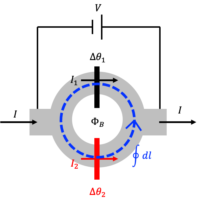
Combine two Josephson junctions \(J_1\) and \(J_2\) to form a closed loop threaded by flux \( \Phi_B \) and subject to voltage \( V \). From the previous section, the loop integral of the superconducting phase must satisfy: \[ \oint \nabla \theta(r) \cdot d\vec{l} - \frac{q}{\hbar} \Phi_B = 2\pi N \] Since the discontinuities at the junctions contribute \( \Delta\theta_1 \) and \( \Delta\theta_2 \), with \( q = -2e \), substitution gives: \[ \Delta\theta_2 - \Delta\theta_1 + 2\pi \frac{\Phi_B}{\Phi_0} = 2\pi N \] \[ \Delta\theta_2 = \Delta\theta_1 - 2\pi \frac{\Phi_B}{\Phi_0} + 2\pi N \]
When current \( I = I_1 + I_2 \) is sent through the entire SQUID, use the Josephson current relation from the previous section. For a symmetric SQUID, the two Josephson junctions have identical properties \( I_c \). We obtain: \[ I = I_1 + I_2 = I_0 (\sin\Delta\theta_1 + \sin\Delta\theta_2) \] \[ I = I_0 \left[\sin\Delta\theta_1 + \sin\left(\Delta\theta_1 - 2\pi \frac{\Phi_B}{\Phi_0} + 2\pi N\right)\right] \] \[ I = I_0 \left[\sin\Delta\theta_1 + \sin\left(\Delta\theta_1 - 2\pi \frac{\Phi_B}{\Phi_0}\right)\right] \] Applying a trigonometric identity gives: \[ I = I_0 \left[2 \sin\left(\frac{\Delta\theta_1 + \Delta\theta_1 - 2\pi \frac{\Phi_B}{\Phi_0}}{2}\right) \cos\left(\frac{\Delta\theta_1 - \Delta\theta_1 + 2\pi \frac{\Phi_B}{\Phi_0}}{2}\right)\right] \] \[ I = 2I_0 \cos\left(\frac{\Phi_B}{\Phi_0} \pi\right) \sin\left(\Delta\theta_1 - \frac{\Phi_B}{\Phi_0} \pi\right) \]
The previous section showed that a Josephson junction behaves inductively; the inductive behavior of a SQUID can be analyzed similarly. Differentiate the current with respect to time: \[ \dot{I} = 2I_0 \cos\left(\frac{\Phi_B}{\Phi_0} \pi\right) \cos\left(\Delta\theta_1 - \frac{\Phi_B}{\Phi_0} \pi\right) \dot{\Delta\theta_1} \] The relation among \( \dot{\Delta\theta_1} \) and voltage \( V \) is: \[ V = \frac{\hbar}{2e} \dot{\Delta\theta_1} = \frac{\Phi_0}{2\pi} \dot{\Delta\theta_1} \] Substitution gives the inductance: \[ L_{\text{SQUID}}(\Delta\theta_1, \Phi_B) = \left[\frac{2\pi}{\Phi_0} \cdot 2I_0 \cos\left(\frac{\Phi_B}{\Phi_0} \pi\right) \cos\left(\Delta\theta_1 - \frac{\Phi_B}{\Phi_0} \pi\right)\right] \]
Notice that \( L_{\text{SQUID}} \) depends on the applied flux \( \Phi_B \). This is the key to frequency tuning in a tunable transmon. Define the variable \( \Phi \): \[ \Phi \equiv \frac{\Delta\theta_1}{\pi} \Phi_0 - \Phi_B = \frac{\Phi_0}{\pi} \left(\Delta\theta_1 - \frac{\Phi}{\Phi_0} \pi\right) \] with: \[ \dot{\Phi} = \frac{\Phi_0}{\pi} \dot{\Delta\theta_1} \] The voltage \( V \) and current \( I \) are respectively: \[ V = \frac{1}{2} \dot{\Phi}, \quad I = 2I_0 \cos\left(\frac{\Phi_B}{\Phi_0} \pi\right) \sin\left(\frac{\Phi}{\Phi_0} \pi\right) \]
At fixed external field \( \Phi_B \), the energy stored in a SQUID is: \[ E = \int IV \, dt = \int \left[2I_0 \cos\left(\frac{\Phi_B}{\Phi_0} \pi\right) \sin\left(\frac{\Phi}{\Phi_0} \pi\right) \cdot \frac{1}{2} \dot{\Phi}\right] dt \] Simplifying gives: \[ E = I_0 \cos\left(\frac{\Phi_B}{\Phi_0} \pi\right) \int \sin\left(\frac{\Phi}{\Phi_0} \pi\right) d\Phi \] \[ E = -\frac{I_0 \Phi_0}{\pi} \cos\left(\frac{\Phi_B}{\Phi_0} \pi\right) \cos\left(\frac{\pi}{\Phi_0} \Phi\right) \]
Tunable Transmon
Frequency-tunable transmon
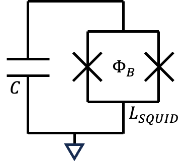
▲ A \(LC\) circuit composed of two Josephson junctions, with tunable inductance.
As discussed above, a Josephson junction has inductive properties, and a transmon is an LC circuit whose inductor is replaced by a Josephson junction. Here we consider a tunable transmon directly, using a SQUID as the inductor. In practice, fabrication nonuniformity gives different transmons different properties. With tunable transmons, small adjustments of magnetic flux \( \Phi_B \) can bring qubit properties into alignment. In addition, when quantizing the LC circuit above, \([ \Phi, Q ] = i\hbar\) formed a canonical pair. The SQUID derivation naturally relates magnetic flux \( \Phi \) to phase difference \( \Delta\theta \): \[ \Phi \equiv \frac{\Delta\theta_1}{\pi} \Phi_0 - \Phi_B \]
We now write the Hamiltonian: \[ \mathcal{H} = \frac{Q^2}{2C} + \frac{\Phi_\#^2}{2L} = \frac{Q^2}{2C} + \frac{(I_0 \pi)}{2\Phi_0} \cos\left(\frac{\Phi_B}{\Phi_0} \pi\right) \Phi^2 - \frac{I_0}{24} \left(\frac{\pi}{\Phi_0}\right)^3 \cos\left(\frac{\Phi_B}{\Phi_0} \pi\right) \Phi^4 + \cdots \] \[ = \frac{Q^2}{2C} + \frac{\Phi^2}{2L} - \frac{1}{24L} \left(\frac{\pi}{\Phi_0}\right)^2 \Phi^4 + \cdots \] where: \[ L = \left(\frac{I_0 \pi}{\Phi_0} \cos\left(\frac{\Phi_B}{\Phi_0} \pi\right)\right)^{-1} \]
We now examine how nonlinearity changes the energy levels. Above, we chose new variables \( a \) and \( a^\dagger \): \[ a = \sqrt{\frac{1}{2\hbar} \sqrt{ \frac{L}{C}}} \left(\sqrt{\frac{C}{L}} \Phi + iQ\right), \quad a^\dagger = \sqrt{\frac{1}{2\hbar} \sqrt{ \frac{L}{C}}} \left(\sqrt{\frac{C}{L}} \Phi - iQ\right) \] Conversely: \[ \Phi = \sqrt{\frac{\hbar}{2 }\sqrt{ \frac{L}{C}}} (a^\dagger + a), \quad Q = i\sqrt{\frac{\hbar}{2} \sqrt{ \frac{C}{L}}} (a^\dagger - a) \]
Expand the Hamiltonian as: \[ \mathcal{H} = \frac{\hbar}{\sqrt{LC}} \left[a^\dagger a + \frac{1}{2}\right] - \frac{1}{24L} \left(\frac{\pi}{\Phi_0}\right)^2 \left[i \sqrt{\frac{\hbar}{2\sqrt{L/C}}} (a^\dagger + a)\right]^4 \] After simplification: \[ \mathcal{H} = \frac{\hbar}{\sqrt{LC}} \left[a^\dagger a + \frac{1}{2}\right] - \frac{\hbar^2}{96C} \left(\frac{\pi}{\Phi_0}\right)^2 (a^\dagger + a)^4 \] This expression contains linear and nonlinear terms. The linear term describes the levels of a quantum harmonic oscillator, while the nonlinear term is the Josephson-junction correction to those levels.
Using perturbation theory, when \( \mathcal{H} = H_0 + \Delta H \), \( \ket{E_0^m} \to \ket{E^m} \), and \( E_0^m \to E^m = E_0^m + \delta E^m \), the correction \( \delta E^m \) to level \( E_0^m \) is:
\[ \delta E^m = \langle E_0^m | \Delta H | E_0^m \rangle = \langle E_0^m | \left[-\frac{\hbar^2}{96C} \left(\frac{\pi}{\Phi_0}\right)^2 (a^\dagger + a)^4\right] | E_0^m \rangle \]
The calculation proceeds as follows:
\[ \langle E_0^m | (a^\dagger + a)^4 | E_0^m \rangle = \langle E_0^m | (aa + aa^\dagger + a^\dagger a + a^\dagger a^\dagger)^2 | E_0^m \rangle \]
Expanding gives:
\[ \langle E_0^m | aa(aa + aa^\dagger + a^\dagger a + a^\dagger a^\dagger) + aa^\dagger(aa + aa^\dagger + a^\dagger a + a^\dagger a^\dagger) + a^\dagger a(aa + aa^\dagger + a^\dagger a + a^\dagger a^\dagger) + a^\dagger a^\dagger(aa + aa^\dagger + a^\dagger a + a^\dagger a^\dagger) \ket{ E_0^m } \]
Because we take an expectation value, only terms with equal numbers of \( a, a^\dagger \) remain:
\[ \langle E_0^m | aaa^\dagger a^\dagger + aa^\dagger aa^\dagger + aa^\dagger a^\dagger a + a^\dagger aaa^\dagger + a^\dagger aa^\dagger a + a^\dagger a^\dagger aa | E_0^m \rangle \]
Continuing to simplify:
\[ \langle E_0^m | a(a^\dagger a + 1)a^\dagger + aa^\dagger aa^\dagger + (a^\dagger a + 1)a^\dagger a + a^\dagger a(a^\dagger a + 1) + a^\dagger aa^\dagger a + a^\dagger (aa^\dagger - 1)a | E_0^m \rangle \]
Rearranging again:
\[ \langle E_0^m | aa^\dagger aa^\dagger + aa^\dagger + aa^\dagger aa^\dagger + a^\dagger aa^\dagger a + a^\dagger a + a^\dagger aa^\dagger a + a^\dagger a + a^\dagger aa^\dagger a + a^\dagger aa^\dagger a - a^\dagger a | E_0^m \rangle \]
Simplifying further:
\[ \langle E_0^m | 2aa^\dagger aa^\dagger + aa^\dagger + 4a^\dagger aa^\dagger a + a^\dagger a | E_0^m \rangle \] \[ = \langle E_0^m | 2(a^\dagger a + 1)(a^\dagger a + 1) + (a^\dagger a + 1) + 4a^\dagger aa^\dagger a + a^\dagger a | E_0^m \rangle \]
Finally, we obtain:
\[ \langle E_0^m | 6a^\dagger aa^\dagger a + 6a^\dagger a + 3 | E_0^m \rangle = 6m^2 + 6m + 3 \]
Define the energy-level spacing:
\[ \Delta E^m_{m-1} = \frac{\hbar}{\sqrt{LC}} - \frac{\hbar^2}{96C} \left(\frac{\pi}{\Phi_0}\right)^2 \left\{6[m^2 - (m-1)^2] + 6\right\} \]
\[ = \frac{\hbar}{\sqrt{LC}} - \frac{\hbar^2 \pi^2}{96C} \frac{e^2}{\pi^2 \hbar^2} \left[6(2m - 1) + 6\right] \]
Finally, we obtain:
\[ \Delta E^m_{m-1} = \frac{\hbar}{\sqrt{LC}} - m\frac{e^2}{8C} \]
Calculate \( \Delta E^{21} - \Delta E^{10} \):
\[ \Delta E^{21} - \Delta E^{10} = \left(\frac{\hbar}{\sqrt{LC}} - 2\frac{e^2}{8C}\right) - \left(\frac{\hbar}{\sqrt{LC}} - \frac{e^2}{8C}\right) \]
\[ = -\frac{e^2}{8C} \equiv -E_C \]
\( E_C \) represents its nonlinear effect.
Ref:
DOI:10.1103/RevModPhys.93.025005
2.3 Types of Superconducting Qubits
Superconducting qubits can be classified into several types according to their dominant energy scales and circuit designs. Common examples include the charge qubit, flux qubit, phase qubit, transmon, fluxonium, and 0–π qubit. In modern gate-based superconducting quantum computing, the transmon is among the most widely used designs; fluxonium has also attracted substantial attention for its long coherence, low relaxation rate, and distinctive level structure.
| Qubit type | Primary degree of freedom | Design features |
|---|---|---|
| Charge Qubit | Cooper pair number | Charge-sensitive, with good controllability but strong susceptibility to charge noise |
| Flux Qubit | Magnetic flux and circulation direction | Based on persistent-current states in a superconducting loop |
| Transmon | Josephson phase | Uses increased capacitance to reduce charge-noise sensitivity |
| Fluxonium | Phase across Josephson junction and superinductor | Uses a superinductor to create a distinctive level structure and noise protection |
Unit 1: Introduction to superconducting quantum-chip layout
1.1 What Is a Superconducting Quantum Chip?
A superconducting quantum chip is a cryogenic quantum circuit fabricated with micro- and nanofabrication processes. Qubits, readout resonators, couplers, control lines, and grounding structures are laid out as specific microwave circuits on the chip. When the chip is cooled to roughly 10 mK to several tens of millikelvin, electrons in the superconducting metal form Cooper pairs and circuit dissipation falls sharply, allowing selected circuit modes to exhibit quantized energy levels.
From an engineering perspective, a superconducting quantum chip is simultaneously a microwave circuit, a cryogenic electronic system, and an artificial quantum system. Understanding it therefore requires quantum mechanics, electromagnetism, circuit theory, materials science, and micro- and nanofabrication.
1.2 Typical Layout Elements
A typical superconducting quantum chip usually contains the following classes of components:
| Chip component | Function | Physical role |
|---|---|---|
| Qubit | Stores and processes quantum information | An artificial atom formed by a nonlinear superconducting circuit |
| Readout Resonator | Reads out the qubit state | A microwave resonator dispersively coupled to the qubit |
| Drive Line | Applies microwave pulses to control the qubit | Produces single-qubit rotations |
| Flux Line | Tunes the frequency of a qubit or coupler | Changes Josephson energy through applied magnetic flux |
| Coupler | Connects two or more qubits | Provides fixed or tunable quantum coupling |
| Ground Plane | Provides an electromagnetic ground reference and shielding | Affects microwave modes, crosstalk, and packaging effects |
| Air Bridge / Crossover | Connects ground planes or crosses signal lines | Suppresses slotline modes and parasitic coupling |
1.3 From Circuit Layout to Hamiltonian
The layout of a superconducting quantum chip is not merely a geometric pattern. It maps to concrete circuit parameters such as capacitance, inductance, coupling strength, resonance frequency, and loss channels. Those parameters in turn determine the system Hamiltonian.
For example, the large metal pads of a transmon set the total capacitance \(C_\Sigma\), the Josephson junction sets the Josephson energy \(E_J\), and together they determine the qubit frequency, anharmonicity, and charge-noise sensitivity.
Core concept
In a superconducting quantum chip, “layout design” is “Hamiltonian engineering.” An apparently geometric design choice ultimately becomes the frequency, coupling, noise sensitivity, and controllability of the quantum system.
Learning Check
- What is the greatest difference between a superconducting quantum chip and a conventional CMOS chip?
- Why must the readout resonator be coupled to the qubit?
- Why does chip layout affect the qubit Hamiltonian?
Classroom Integration and Assessment
Discussion question: Given \(f_{01}\) and a target anharmonicity, estimate \(E_C\), \(E_J\), the total capacitance, and \(I_c\); then explain where the approximation may fail.
Completion criterion: Students must leave a checkable derivation, relationship diagram, comparison table, or architecture decision, and must be able to explain its physical assumptions and engineering costs.
Core and Further Reading
- Charge-insensitive Qubit Design Derived from the Cooper Pair BoxJ. Koch et al., Physical Review A 76, 042319 (2007).The trade-off among transmon \(E_J/E_C\), charge dispersion, and anharmonicity.
- A Quantum Engineer's Guide to Superconducting QubitsP. Krantz et al., Applied Physics Reviews 6, 021318 (2019).A foundational review of control, coherence, readout, and engineering parameters.
- Engineering High-Coherence Superconducting QubitsI. Siddiqi, Nature Reviews Materials 6, 875–891 (2021).Design trade-offs among different qubit architectures, material loss, and coherence.
- Mitigation of Frequency Collisions in Superconducting Quantum ProcessorsJ. B. Hertzberg et al., Physical Review Research 5, 043001 (2023).How process variation becomes qubit-frequency spread, collisions, and yield loss.
Reverse-engineering assignment: infer the artificial atom from a chip image
Assignment question: Given a local image of a superconducting quantum chip, can you infer the Hamiltonian it might implement from the geometry?
- Identify the structures: Mark the qubit pads, Josephson junction, ground, drive line, and readout resonator; explicitly label any uncertain identification.
- geometry → parameter: Explain which circuit parameters are affected by pad geometry, junction area, spacing, and line length.
- parameter → Hamiltonian: Identify which structures in the image primarily control \(E_C\), \(E_J\), and the coupling term.
- Hamiltonian → observable: Predict how \(f_{01}\), anharmonicity, charge dispersion, or coupling changes when the pads grow larger, the junction becomes smaller, or the resonator is moved closer.
- Limits of inference: List the information that cannot be known from an image alone and must come from process data, EM simulation, or experimental measurement.
Assignment throughline: Chip structure → geometric parameters → lumped-element model → Hamiltonian term → spectrum/control hypothesis. This is a reverse-design problem with explicit evidentiary limits; students are not expected to infer the complete system architecture in W2.