PHYS598500 · Week 1 · T1A
Computation Is Physical
From Mechanized Reasoning to Quantum Hardware and the Limits of Physics
Week Overview
Seven Questions for the First Lecture
- Can calculation and reasoning be mechanized?
- What can a machine compute?
- Why quantum computing if classical computers are already universal?
- Why must reversible computation meet quantum dynamics?
- Must quantum computation be expressed as a sequence of gates?
- How does a computational model become hardware, and what ultimately limits it?
- Can a machine completely describe, predict, and reproduce itself?
Learning Outcomes
- Distinguish a function, an algorithm, a model of computation, a machine architecture, and a physical implementation.
- Separate computability from complexity and explain what quantum computation changes.
- Derive why a many-to-one Boolean map needs reversible embedding before it can be implemented by closed quantum evolution.
- Compare gate-based, measurement-based, and adiabatic computation through their physical resources and control primitives.
- Trace a computation from abstract specification to Hamiltonian, controls, measurement records, and fundamental physical limits.
- Explain how self-reference produces formal limits, while encoded descriptions make self-reproducing machines possible.
Q1. Can Calculation and Reasoning Be Mechanized?
From Human Procedure to Symbolic State Transformation
The First Separation: Answer versus Procedure
A mathematical relation such as (f(x)=y) specifies which answer is correct. A computation additionally specifies a finite procedure that produces the answer. Mechanization begins when the procedure can be followed without further insight at each step.
Ask the class: Which part of long division requires understanding, and which part only requires obeying rules?
Once a task is expressed as explicit state transitions, a person, a gear train, a relay network, or a transistor circuit may carry out the same formal procedure.
\[\text{problem}\rightarrow\text{representation}\rightarrow\text{procedure}\rightarrow\text{state transitions}\rightarrow\text{physical execution}.\]
What Does “Mechanical Computation” Mean?
“Mechanical” does not require metal gears. It means that, once the input and rules are supplied, each next step can be determined without asking the executor for a new mathematical insight.
A human following a table, a relay circuit, a transistor processor, and a simulated Turing machine can all perform mechanical computation. Their materials differ; the relevant common structure is an explicitly specified transition from one configuration to the next.
\[\boxed{\text{current configuration}+\text{rule}\longrightarrow\text{next configuration}.}\]
| Instruction | Mechanical? | Reason |
|---|---|---|
| “Add the two digits and carry according to this table.” | Yes | The next action is completely specified. |
| “Try all divisors from 2 through \(\lfloor\sqrt N\rfloor\).” | Yes | Potentially slow, but finite and explicit. |
| “Find an elegant proof.” | No | Neither the search steps nor a stopping rule are specified. |
| “Guess a useful substitution.” | Not yet | It becomes mechanical only after a precise selection procedure is supplied. |
The Five Ingredients of a Mechanical Computation
- Representation: Which physical or symbolic states stand for the input, workspace, and output?
- Configuration: What information completely describes the machine at one instant?
- Transition rule: Given the current configuration, which next configurations are allowed?
- Control: Which rule is applied next, and can data alter that choice?
- Termination and readout: How do we recognize completion and interpret the resulting state?
For a deterministic digital machine, one may summarize a step as
\[(s_t,x_t)\mapsto(s_{t+1},y_t).\]
The symbols do not move themselves. A physical machine must encode \(s_t\) and \(x_t\), generate the transition, stabilize the result against noise, and expose \(y_t\) for later use.
Worked Example: Mechanizing Euclid's Algorithm
To calculate \(\gcd(a,b)\) for positive integers, repeat:
\[(a,b)\mapsto(b,\;a\bmod b)\]
until \(b=0\); then output \(a\). For \((a,b)=(48,18)\):
\[(48,18)\rightarrow(18,12)\rightarrow(12,6)\rightarrow(6,0),\qquad\gcd(48,18)=6.\]
No step requires the executor to understand why the algorithm works. The proof of correctness belongs to the algorithm designer; execution requires only comparison, remainder, assignment, repetition, and a stopping test.
Mechanization Check
Identify the representation, current configuration, transition rule, control condition, halting state, and output interpretation in this example.
Mechanization, Automation, and Programmability
| Concept | Meaning | Example |
|---|---|---|
| Mechanization | Express a task as explicit elementary state transitions. | Euclid's algorithm written as repeatable rules |
| Automation | Arrange for a physical system to execute those transitions with little or no intervention. | A calculator repeatedly updating registers |
| Programmability | Allow the same machine to execute different procedures by changing an encoded program. | A stored-program computer |
| Universality | Allow one model to simulate every computation in a specified class. | A universal Turing machine |
A clockwork calculator can be automatic without being general-purpose. A modern processor is programmable, but a particular program may still fail to halt. These distinctions prepare Q2: after a procedure is mechanized, we can ask what any such mechanism can compute.
A Short Intellectual Arc
| Step | What became mechanical? | What remained to be specified? |
|---|---|---|
| Abacus and mechanical calculators | Arithmetic operations | Which operations and in what order |
| Babbage's Difference Engine | Repeated numerical tabulation | How to make one machine programmable |
| Babbage's Analytical Engine | A general architecture of memory, operations, and control | How to express programs and uses beyond arithmetic tables |
| Ada Lovelace's Notes | A machine-directed algorithm and a broader concept of symbolic manipulation | Which problems can be encoded for the machine |
| Boolean algebra | Logical propositions as algebraic symbols | How symbols are physically represented |
| Logic circuits | Rules as networks of elementary operations | Sequencing, memory, and control |
| Stored-program machines | The operation sequence itself becomes data | Resources, errors, and physical realization |
Historical caution: machines existed before Boolean and Turing. The conceptual advance was not the first hardware, but a precise language for what can be mechanized and made universal.
Charles Babbage: From Automatic Tables to a Programmable Machine
Charles Babbage (1791–1871) first designed the Difference Engine to automate numerical tables. Finite differences reduce polynomial tabulation to repeated addition, making the task suitable for a gear-based mechanism and reducing human calculation and typesetting errors.
The later Analytical Engine was a general architecture. It separated a “store” from a “mill,” used punched cards to specify operations and data, and included sequencing, repetition, and conditional control.
| Design | Modern analogy |
|---|---|
| Store | Memory |
| Mill | Arithmetic/processing unit |
| Punched cards | Program and data input |
| Operation sequence | Control flow |
Caution: the full Analytical Engine was not completed in Babbage's lifetime.
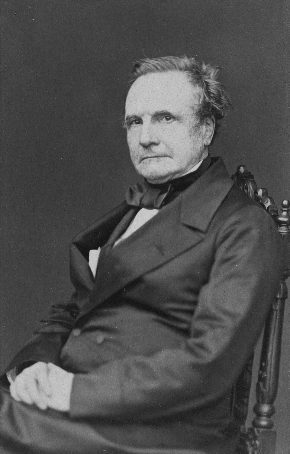
Why Mechanize Tables? Checking Still Failed
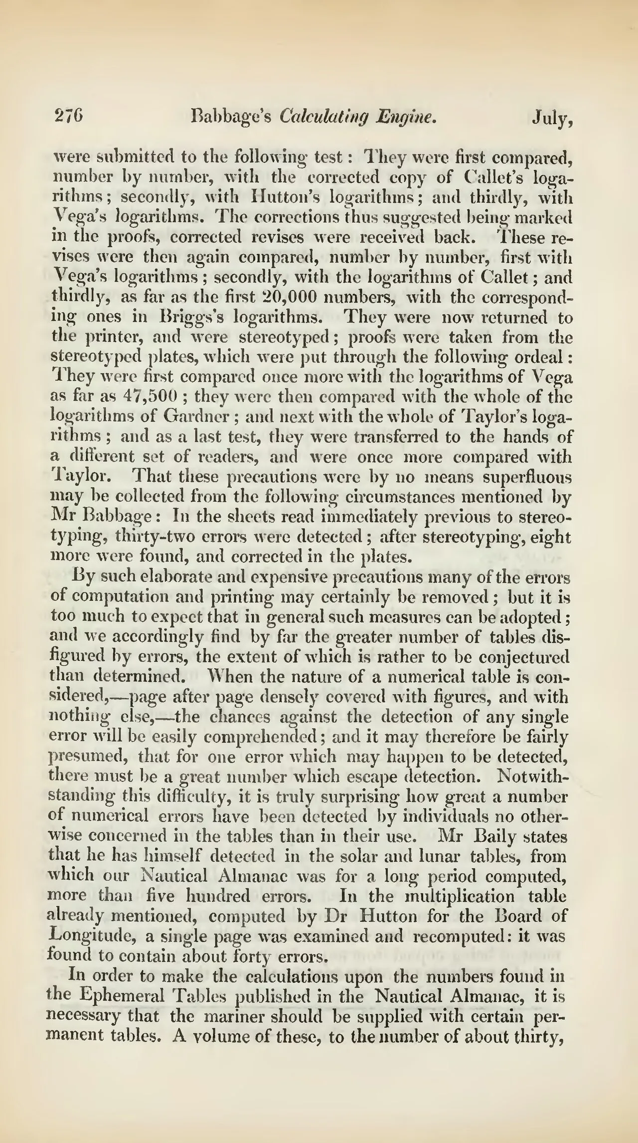
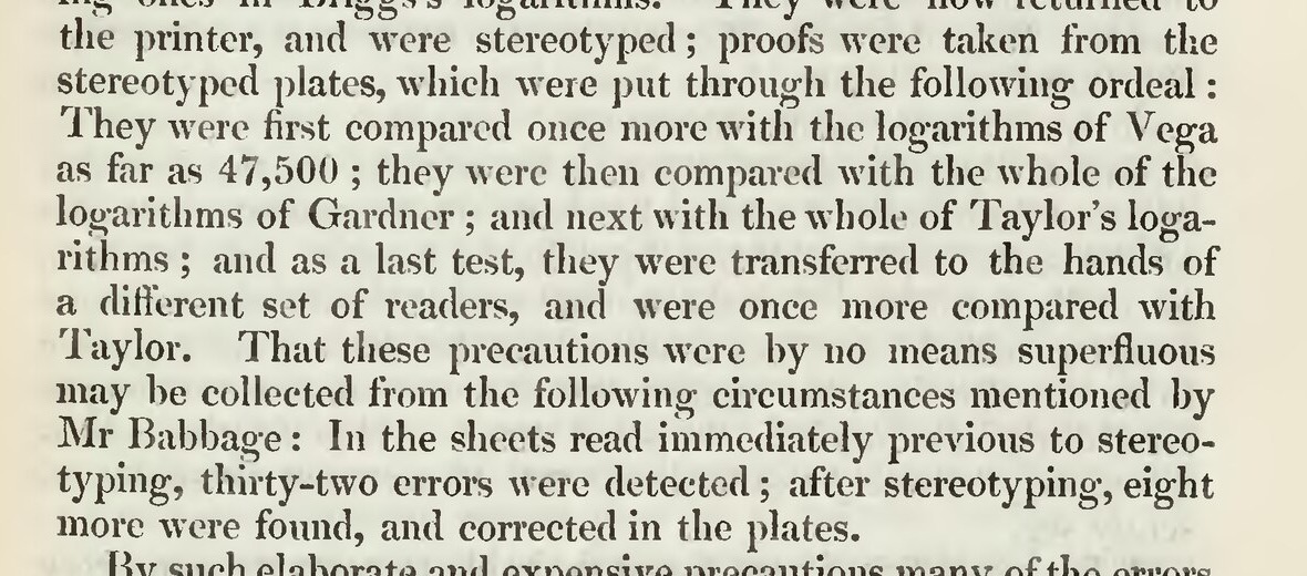
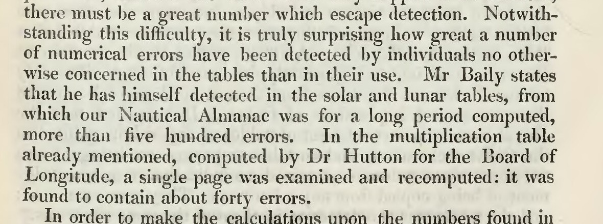
The Table Crisis: “Errata upon Errata”
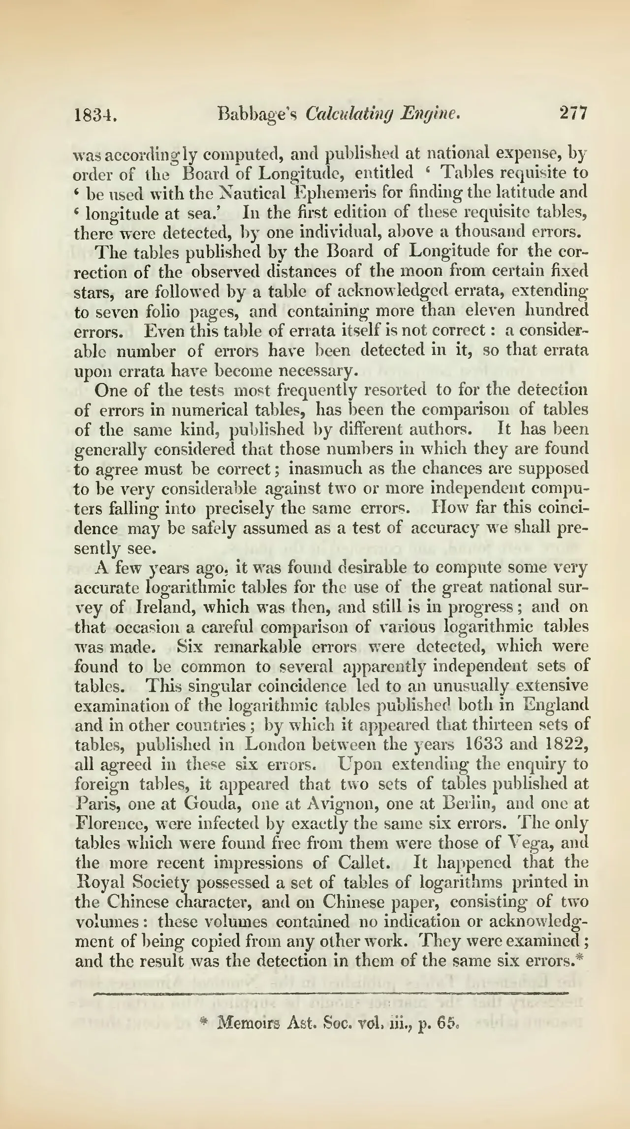
The Edinburgh Review, vol. 59 · July 1834
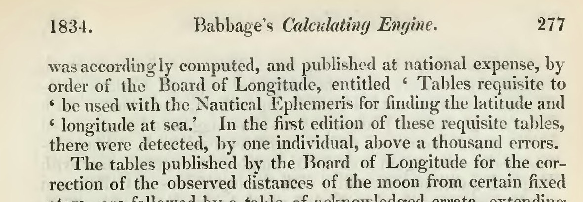
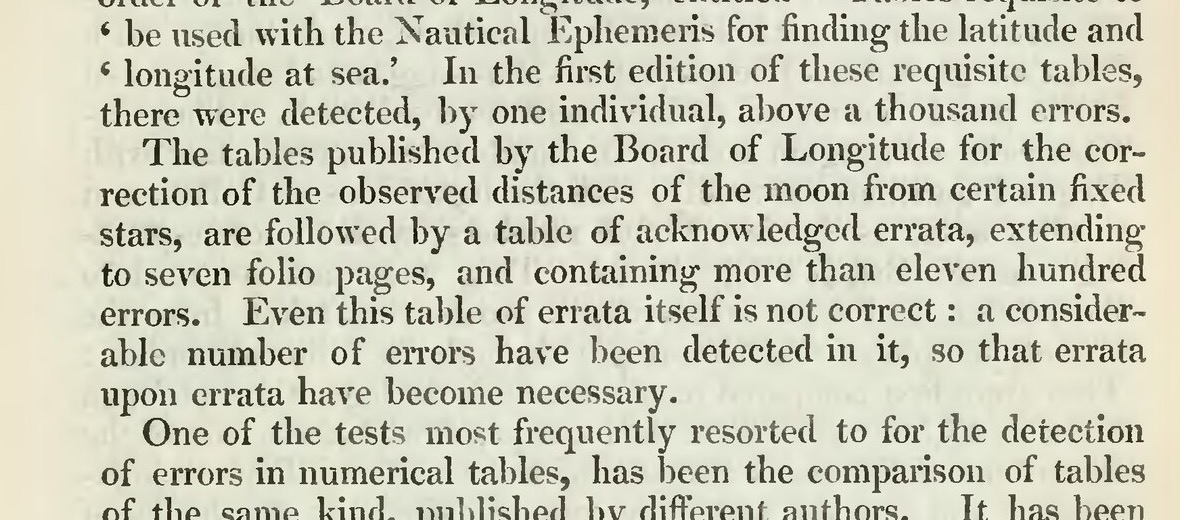
Same Page, Two Copied Errors: Hutton vs. Babbage
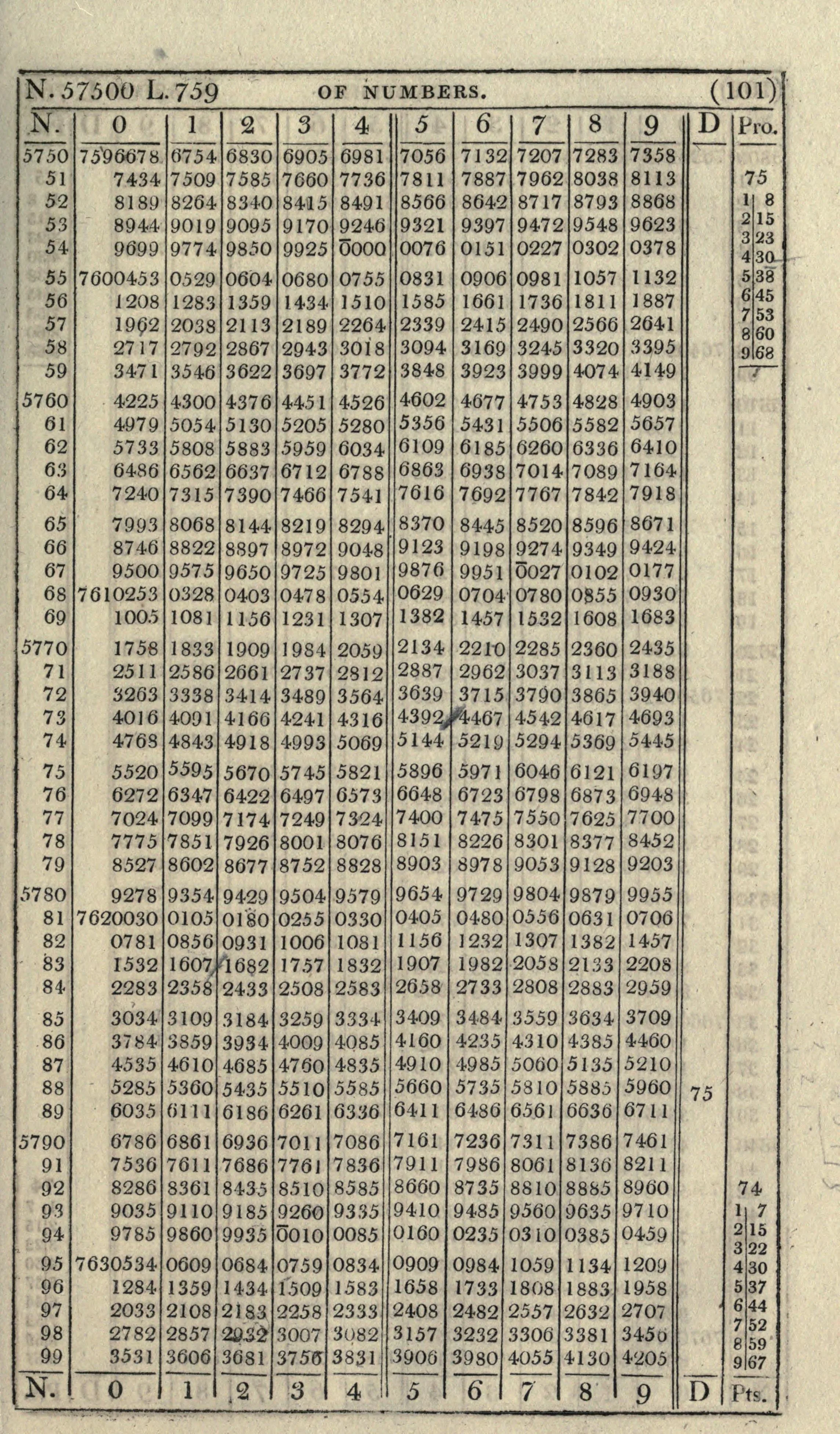
 wrong
wrong
57,628 → …633657,629 → …6410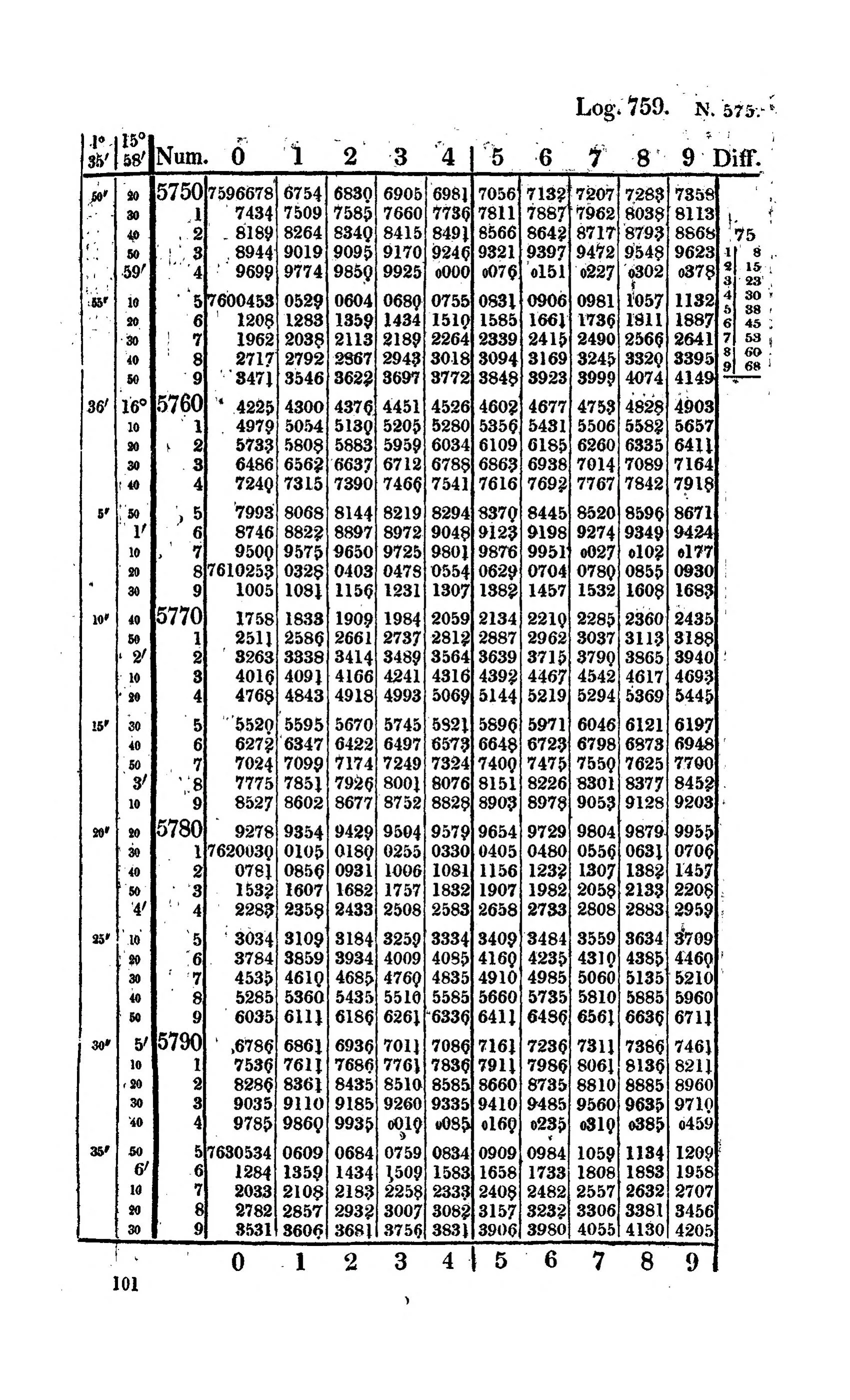
 correct
57,628 → …633557,629 → …6411Difference Engine No. 2: Built in Metal
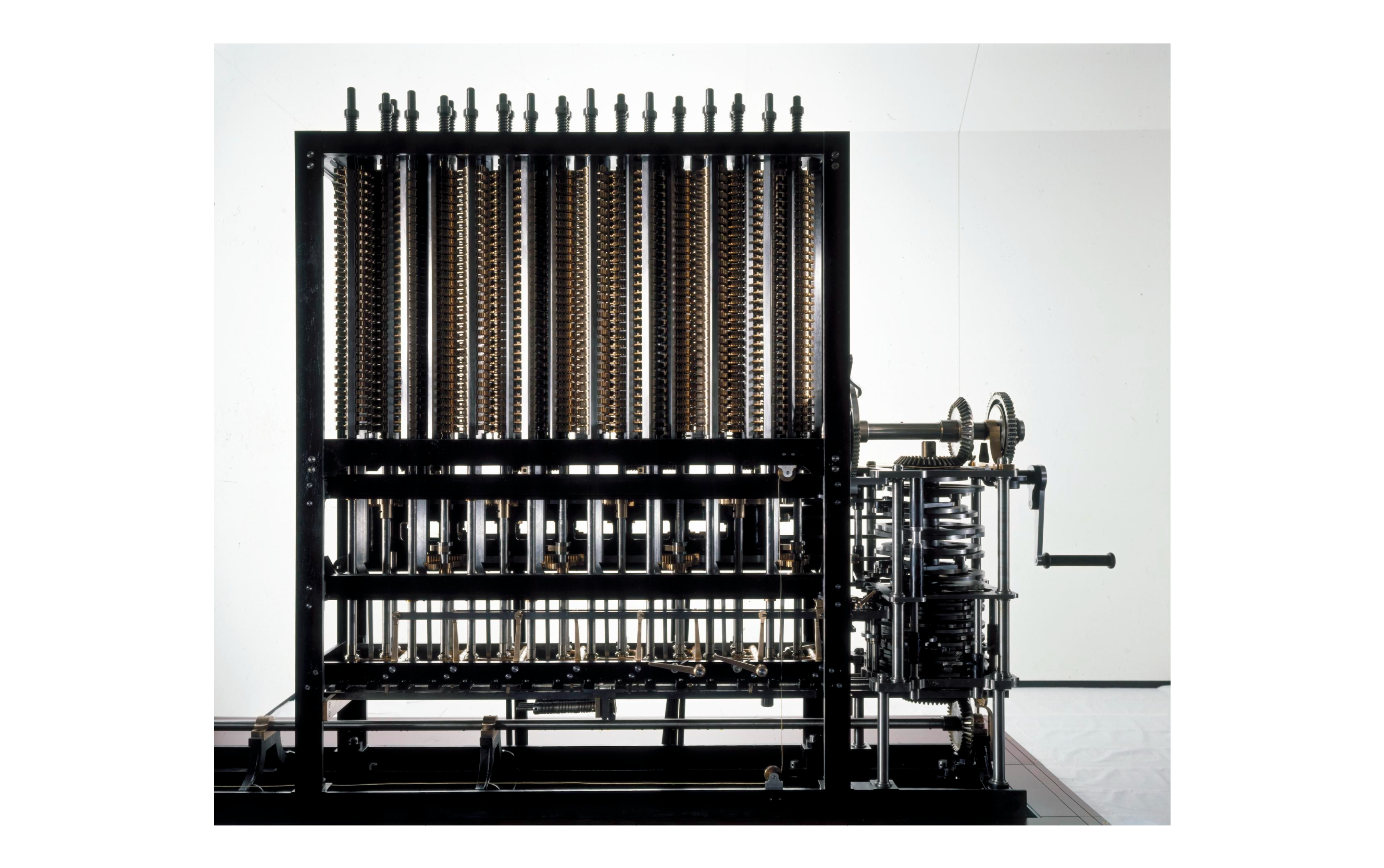
Complete reconstruction
Ref:
Science Museum Group Collection
▲
Ref:
https://collection.sciencemuseumgroup.org.uk/objects/co62748/babbages-difference-engine-no-2-2002
拷貝.png)
Decimal figure wheels and gear trains
Ref:
Science Museum Group Collection
▲
Ref:
https://collection.sciencemuseumgroup.org.uk/objects/co62748/babbages-difference-engine-no-2-2002
Difference Engine No. 2: From Drawings to Mechanism
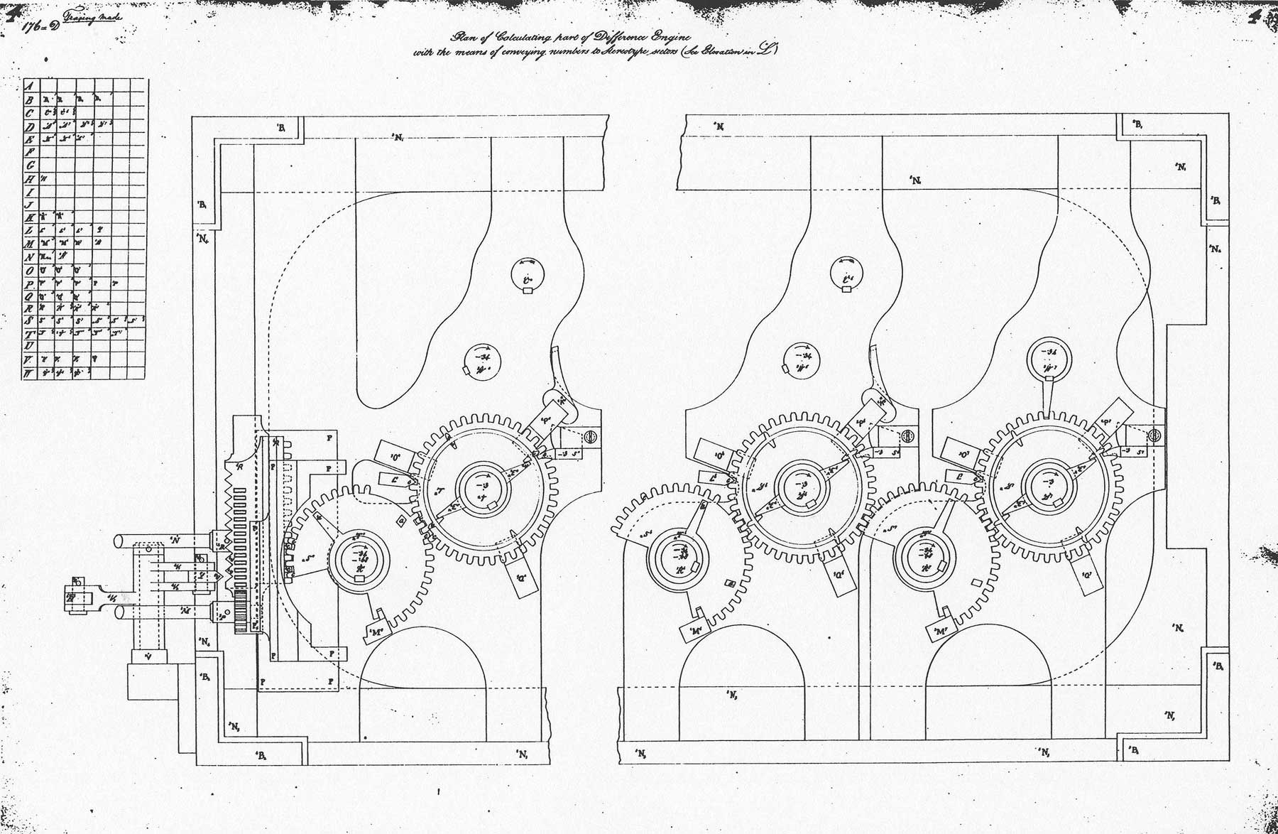
Plan of the calculating mechanism
Ref:
Cronatec · How did the Difference Engine work?
▲
Ref:
https://cronatec.ch/how-did-the-difference-engine-work/
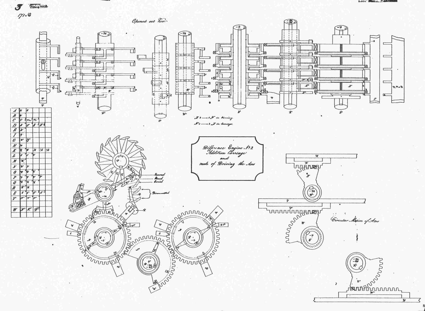
Addition and carriage mechanisms
Ref:
Cronatec · How did the Difference Engine work?
▲
Ref:
https://cronatec.ch/how-did-the-difference-engine-work/
Why the Analytical Engine Was a Conceptual Breakthrough
The Difference Engine mechanized a specialized mathematical task. The Analytical Engine asked a deeper question: can the same machine perform many tasks when its sequence of operations is changed?
\[\boxed{\text{fixed-purpose mechanism}\rightarrow\text{programmable general-purpose architecture}.}\]
This anticipates three distinctions that remain essential:
- Machine: the physical system and its available elementary operations.
- Program: an encoded sequence that selects and organizes those operations.
- Data: the encoded objects on which the operations act.
Babbage did not build a functioning modern computer, and the Analytical Engine was not a Turing machine formulated a century early. Its importance is architectural: it made programmable, automatic symbolic procedure imaginable as a machine design.
Analytical Engine: Mechanism and Punched-Card Control

Ref: Science Museum Group Collection
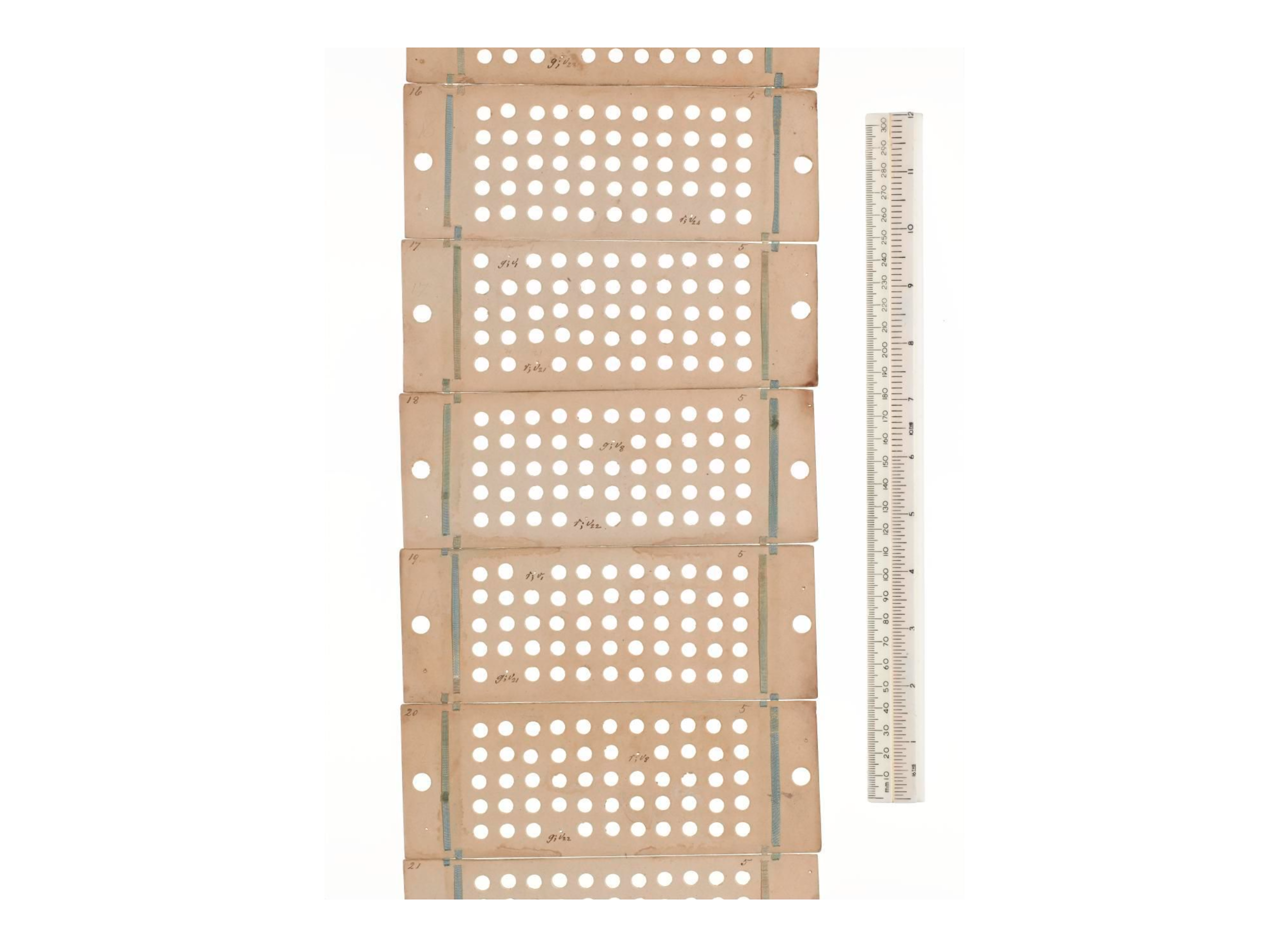
Ref: Science Museum Group Collection
Ada Lovelace: Her Contribution, Precisely
Publication and analysis: Ada Lovelace (1815–1852) translated Luigi Menabrea's account and added Notes A–G—the most extensive contemporary published explanation of how the Engine could be directed.
Machine-directed algorithm: she expressed a complete procedure as ordered operations, variables and storage locations, intermediate states, sequencing, and repetition—the form required for machine execution.
Machine–program distinction: the mechanisms provide general operations; an encoded card sequence determines the particular procedure and data flow.
General account of computation: formally represented relations could be subjected to rule-governed symbolic manipulation, extending the idea of automatic calculation.
Historical precision: Babbage designed the architecture; “first programmer” is debated. Lovelace's clearest contribution was articulating machine-directed programming and symbolic computation.
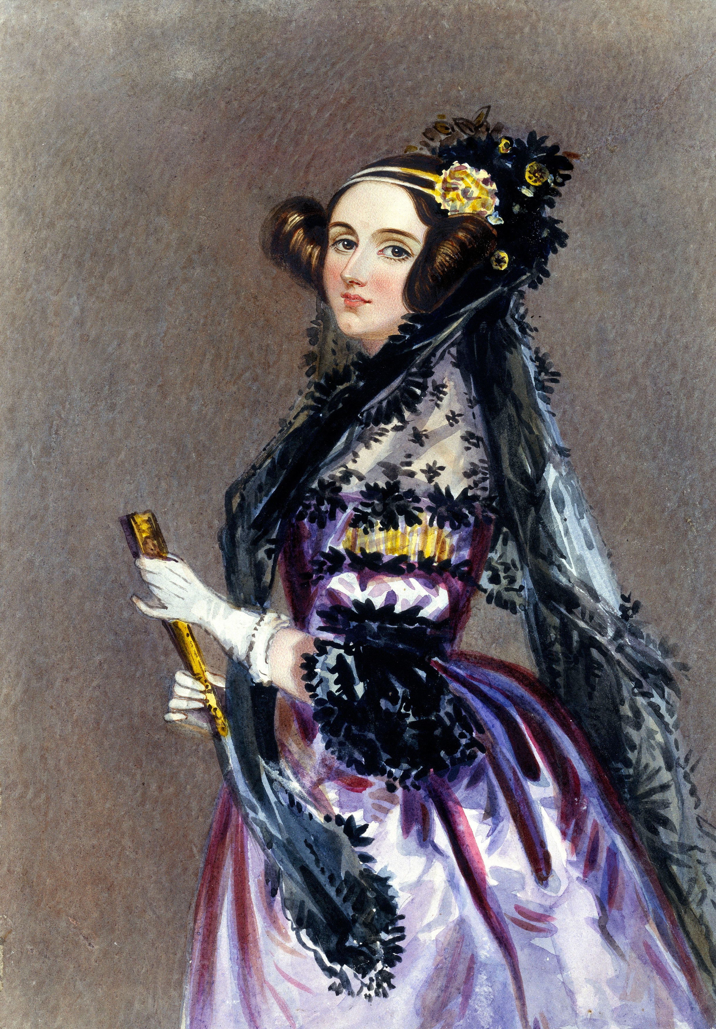
Babbage and Lovelace Ask Different Questions
| Question | Babbage's contribution | Lovelace's contribution |
|---|---|---|
| What machine could execute a procedure? | Store, mill, cards, and control architecture | Interpreted how procedures would inhabit that architecture |
| How is a calculation represented? | Mechanical operations on encoded numbers | Tables of variables, operations, and intermediate states |
| What could such a machine manipulate? | General numerical operations | Potentially any formally representable relations |
| Where does novelty come from? | The machine executes supplied rules | The human supplies representations, rules, and objectives |
Discussion Prompt
Is the Analytical Engine important because it could calculate faster, or because it separated hardware from an encoded program? Which of those two ideas survives most directly in quantum computing?
Two Lines Converge into the Modern Computer
A conceptual map of converging ideas—not a claim of one linear chronology or direct personal influence.
Boole: Logic Becomes Algebra
George Boole was not designing a computer. His contribution was to show that logical relations could be represented by symbols and transformed according to algebraic rules.
For Boolean variables \(a,b\in\{0,1\}\):
\[a\land b,\qquad a\lor b,\qquad\neg a.\]
For example, “the machine starts only if a key is present and the button is pressed” becomes
\[\mathrm{start}=\mathrm{key}\land\mathrm{button}.\]
This separates the logical relation from the material that represents it. The same Boolean expression may later be realized using relays, vacuum tubes, transistors, fluidic valves, or other two-state devices.
Boole supplied a language for logic, not the engineering bridge to digital circuits. That bridge arrives with switching theory.
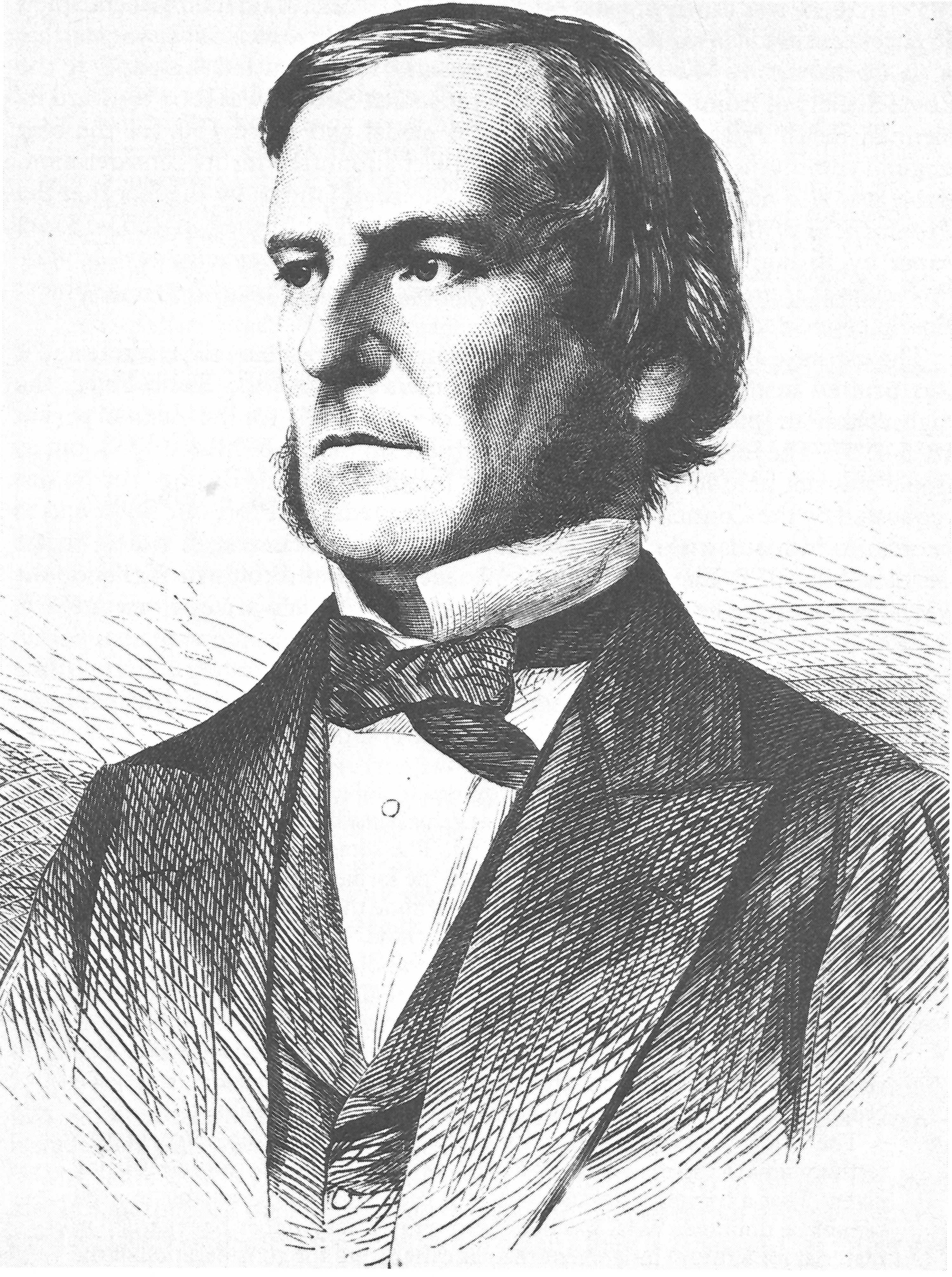
George Boole
Ref:
Wikipedia
Shannon: Boolean Algebra Becomes Switching-Circuit Design
Claude Shannon (1916–2001) showed that relay switching networks could be analyzed and synthesized using Boolean algebra. A relay contact supplies two distinguishable states that may encode \(0\) and \(1\).
| Connection | Boolean operation |
|---|---|
| Normally open contacts in series | \(a\land b\) |
| Contacts in parallel | \(a\lor b\) |
| Normally closed contact controlled by \(a\) | \(\neg a\) |
\[\boxed{\text{Boolean expression}\longleftrightarrow\text{switching network}.}\]
This made circuit design systematic: formulate a truth table, derive and simplify a Boolean expression, then construct a switching network with the same relation.
.jpg)
Worked Bridge: From Addition to a Boolean Circuit
A half adder accepts two bits and returns a sum bit and a carry bit:
| \(a\) | \(b\) | sum \(s\) | carry \(c\) |
|---|---|---|---|
| 0 | 0 | 0 | 0 |
| 0 | 1 | 1 | 0 |
| 1 | 0 | 1 | 0 |
| 1 | 1 | 0 | 1 |
The truth table gives
\[s=a\oplus b,\qquad c=a\land b.\]
Thus arithmetic meaning has been translated into a binary representation, then into Boolean functions, and finally into XOR and AND switching networks.
Carry Makes Multi-Bit Addition a Sequential Architecture Problem
A full adder also accepts the previous column's carry \(c_i\):
\[s_i=a_i\oplus b_i\oplus c_i,\]
\[c_{i+1}=(a_i\land b_i)\lor\left[c_i\land(a_i\oplus b_i)\right].\]
Connecting full adders produces a ripple-carry adder:
\[c_0\rightarrow\mathrm{FA}_0\rightarrow c_1\rightarrow\mathrm{FA}_1\rightarrow\cdots\rightarrow c_n.\]
This single example combines all the historical contributions:
- mechanical procedure: add one column, save carry, move left;
- Boolean representation: express sum and carry as functions of bits;
- switching realization: implement the functions with physical gates;
- architecture: connect gates, retain state, and control their order.
From Gears to Integrated Circuits
| Stage | Physical representation | Concept retained |
|---|---|---|
| Babbage's mechanisms | Decimal gear positions | Store, operation, sequence, carry |
| Electromechanical relays | Open/closed contacts | Boolean switching networks |
| Vacuum-tube computers | Electronic conduction states | Faster logical switching |
| Transistor computers | Controlled semiconductor current | Compact, reliable gates |
| Integrated circuits | Many transistors on one substrate | Processors, registers, and memory at scale |
The physical carrier changed radically, but the abstraction survived:
\[\text{encoded state}\rightarrow\text{allowed operation}\rightarrow\text{new encoded state}.\]
One Rule across Five Layers
Consider \(y=(a\land b)\lor(\lnot c)\). It may be represented as:
- a sentence about a decision;
- a Boolean expression;
- a truth table;
- a network of AND, OR, and NOT gates;
- voltages and currents in a transistor network.
\[\boxed{\text{reasoning}\rightarrow\text{symbolic rules}\rightarrow\text{Boolean algebra}\rightarrow\text{logic circuit}\rightarrow\text{physical machine}}\]
Opening Diagnostic
At which arrow do time, energy, noise, and failure first enter? Defend your answer.
Resolution
The abstract layers do not assign numerical energy or error costs, but every executable representation already assumes a physical carrier. The costs become explicit at implementation; they were never absent. This distinction—formal equivalence versus physical cost—will recur in every quantum-computing model.
Transition: If reasoning can be decomposed into mechanical steps, can every well-posed question be solved by some machine?
What Makes a Procedure Mechanical?
A mechanical procedure must specify a finite description of its symbols and rules, a determinate next step for every allowed configuration, and a recognizable stopping condition. “Find a clever factorization” is a goal; trial division is a procedure.
| Property | Question | Failure example |
|---|---|---|
| Effective step | Can the step be executed without new insight? | “Guess the right lemma” |
| Finite description | Can the rules be encoded finitely? | An infinite lookup table |
| Determinacy | Is the next legal action specified? | An unresolved instruction |
| Termination | Does the procedure halt on the promised domain? | An uncontrolled search |
Nondeterministic and probabilistic models modify the form of the transition rule, but they still require a precise mathematical specification.
Boolean Algebra as a Representation of Decisions
For \(a,b\in\{0,1\}\), Boolean operations satisfy identities that permit symbolic simplification:
\[a\land1=a,\quad a\lor0=a,\quad a\lor(a\land b)=a,\quad \neg(a\land b)=\neg a\lor\neg b.\]
The importance is not that nature “thinks in Boolean algebra.” It is that logical propositions can be encoded into a finite algebra whose operations can be mapped to devices with two distinguishable states.
Worked Simplification
Show that \((a\land b)\lor(a\land\neg b)=a\) by algebra, truth table, and a circuit whose two branches recombine. The three representations have identical semantics but different physical costs.
Combinational Logic Is Not Yet a Computer
A combinational circuit maps present inputs to present outputs. A computer also needs state and sequencing. A clocked register supplies memory; a finite-state controller chooses the next operation; conditional branches let data affect control flow.
\[s_{t+1}=F(s_t,x_t),\qquad y_t=G(s_t,x_t).\]
This equation already resembles dynamics: a machine is described by a state and an update law. Quantum hardware will preserve this architectural question while replacing classical state space and allowed updates.
- Combinational logic: no retained history.
- Sequential logic: state persists across steps.
- Stored program: instructions and data share an encodable memory.
Worked Example: A One-Bit Full Adder
Inputs \(a,b,c_{\mathrm{in}}\) produce
\[s=a\oplus b\oplus c_{\mathrm{in}},\qquad c_{\mathrm{out}}=(a\land b)\lor(c_{\mathrm{in}}\land(a\oplus b)).\]
At the semantic layer this is integer addition. At the circuit layer it is XOR/AND/OR. At the CMOS layer each logical operation expands into transistors, capacitances, delays, and switching energy. At the architecture layer many adders form an arithmetic unit, but carry propagation introduces a depth cost.
Resource Question
Which facts are visible in the equations, and which require knowing the circuit topology and device technology?
Q2. What Can a Machine Compute?
Computability, Complexity, and Universality
Alan Turing: A Minimal Universal Model of Computation
Babbage supplied architecture, Boole supplied symbolic logic, and Shannon supplied switching realization. Alan Turing (1912–1954) asks the general question: what counts as a mechanically executable computation, independent of technology?
A Turing machine uses finite control rules, readable and writable memory, and discrete transitions:
\[(q,s)\mapsto(q',s',d),\qquad d\in\{L,R\}.\]
Its importance is not paper tape, but a precise model of mechanical procedure. A universal Turing machine receives the description of another machine as input and simulates it:
\[U(\langle M,x\rangle)=M(x).\]
The same machine performs different tasks because the encoded program changes.
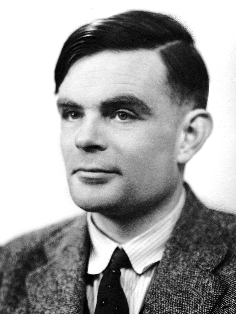
Three Questions That Must Not Be Confused
| Question | Meaning | Typical language |
|---|---|---|
| Computability | Does any terminating algorithm exist? | Computable / undecidable |
| Complexity | How do time and memory scale with input size? | (T(n)), (S(n)), efficient / intractable |
| Universality | Can one programmable model simulate all computations in a target class? | Universal machine / universal gate set |
\[\boxed{\text{Computability asks whether; complexity asks at what cost.}}\]
Universality Does Not Mean Omnipotence
The halting problem gives a boundary: there is no general algorithm that correctly decides for every program and input whether that program eventually stops. A universal computer can simulate every computable procedure; it cannot decide every mathematically expressible question.
Quantum computing is not normally expected to turn uncomputable functions into computable ones. Its central promise is different: the physical model can change the resources required for some computable tasks.
Classification Check
Classify each claim: (a) no algorithm exists; (b) an algorithm requires exponential time; (c) one instruction set approximates every unitary; (d) a processor runs many programs.
The Minimum Architecture Vocabulary
Any executable model must identify:
\[\boxed{\text{representation}+\text{memory}+\text{allowed operations}+\text{control flow}+\text{input/output}.}\]
This is enough architecture for Week 1. Later we will ask the same five questions of a circuit computer, a measurement-based photonic computer, and an adiabatic processor.
Transition: If classical machines are already universal, what could changing the underlying physics possibly add?
The Convergence into the Modern Digital Computer
| Contribution | Question answered | Modern inheritance |
|---|---|---|
| Babbage | How can one machine organize memory, operations, and control? | Programmable architecture |
| Lovelace | How can a procedure be expressed for that machine? | Programs, variables, iteration, symbolic use |
| Boole | How can logical relations become algebra? | Boolean functions |
| Turing | What is a mechanically computable procedure? | Computability and universal simulation |
| Shannon | How can Boolean functions become physical switching networks? | Digital logic design |
| Stored-program architecture | How can instructions and data inhabit electronic memory? | General-purpose electronic computers |
\[\boxed{\text{programmable architecture}+\text{formal computation}+\text{Boolean switching}+\text{stored program}.}\]
“Von Neumann architecture” is useful shorthand, but the stored-program electronic computer emerged from multiple contributors and wartime/postwar projects. Present it as a convergence, not a single-person invention.
A Formal Turing-Machine Configuration
A deterministic Turing machine can be specified by \(M=(Q,\Sigma,\Gamma,\delta,q_0,q_{\mathrm{acc}},q_{\mathrm{rej}})\). A configuration contains the internal state, tape contents, and head position. The transition function is
\[\delta:(Q\setminus\{q_{\mathrm{acc}},q_{\mathrm{rej}}\})\times\Gamma\rightarrow Q\times\Gamma\times\{L,R\}.\]
This formalism separates the machine definition from its physical implementation. Paper tape, magnetic domains, semiconductor memory, and simulated arrays may realize the same transition system with very different resource costs.
Universal Simulation and Program as Data
A universal machine \(U\) receives an encoding \(\langle M,x\rangle\) and simulates machine \(M\) on input \(x\):
\[U(\langle M,x\rangle)=M(x).\]
The conceptual leap is that an instruction sequence is itself information. This makes compilers, interpreters, virtual machines, and programmable processors possible. Universality is model-relative: a universal Boolean gate set, a universal quantum gate set, and universal adiabatic computation refer to the class of transformations each model can approximate or simulate.
Why the Halting Problem Is Undecidable
Assume a program \(H(P,x)\) decides whether \(P(x)\) halts. Construct \(D(P)\): if \(H(P,P)\) predicts halt, loop forever; otherwise halt. Now evaluate \(D(D)\). Either prediction contradicts the behavior that \(D\) was defined to perform.
\[D(D)\text{ halts}\iff H(D,D)=\text{does not halt}\iff D(D)\text{ does not halt}.\]
The lesson is not that ordinary programs are hopeless. It is that even a universal computer has logical limits independent of processor speed.
Quantum computation does not remove this diagonal contradiction: changing amplitudes and gates does not provide a general halting oracle.
Complexity Requires a Cost Model
Let input length be \(n\). A time bound counts elementary steps; a space bound counts simultaneously used memory. Polynomial and exponential examples are
\[T_1(n)=n^3,\qquad T_2(n)=2^n.\]
Asymptotic notation suppresses constants, but hardware feasibility cannot. A quantum resource estimate may require logical qubits, circuit depth, T count, T depth, error-correction cycles, connectivity, classical decoding latency, and total failure probability.
Complexity theory compares idealized models; engineering translates those counts into seconds, joules, devices, cables, calibration time, and money.
Church–Turing versus Physical Church–Turing Theses
The Church–Turing thesis identifies effectively calculable functions with Turing-computable functions. It is not an ordinary mathematical theorem because “effective calculability” begins as an informal concept.
A stronger efficiency claim—the extended or physical Church–Turing thesis—roughly proposes that physically reasonable computation can be efficiently simulated by a probabilistic classical machine. Quantum algorithms challenge this efficiency claim, not the basic set of computable functions.
State this carefully: complexity separations involving realistic quantum advantage depend on unproved assumptions. Shor gives a polynomial-time quantum algorithm; it does not prove that no polynomial-time classical factoring algorithm exists.
Q3. Why Quantum Computing If Classical Computers Are Already Universal?
Feynman's Simulation Challenge and Shor's Complexity Shock
Feynman's Question: Can Nature Efficiently Simulate Itself?
An arbitrary pure state of (n) two-level systems is
\[|\psi\rangle=\sum_{x\in\{0,1\}^n}\alpha_x|x\rangle,\qquad \sum_x|\alpha_x|^2=1.\]
A direct classical description contains (2^n) complex amplitudes. This does not prove that every quantum system is classically hard to simulate—structure, symmetry, sparsity, and approximation can help—but it identifies a serious scaling problem for generic many-body dynamics.
Feynman's proposal reverses the strategy: rather than forcing a classical machine to track every amplitude, construct a controllable quantum system whose own evolution represents the target dynamics.
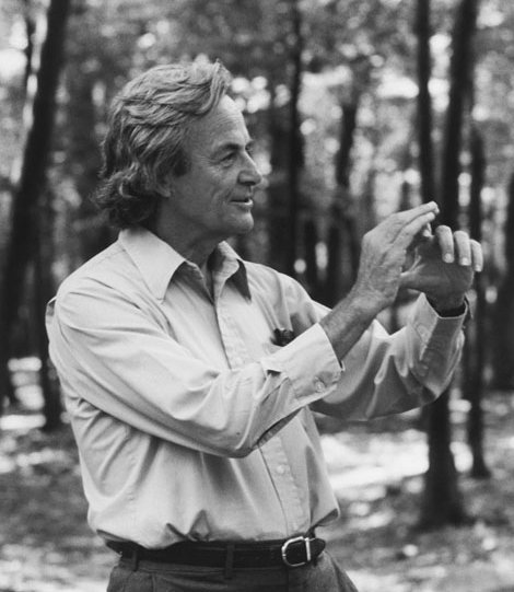
Richard Feynman
Ref:
Wikipedia
Shor's Shock: Quantum Advantage Is Not Limited to Simulating Physics
Integer factoring is computable on a classical computer. Shor's algorithm did not change its computability; it changed the known asymptotic resource scaling by exploiting quantum period finding.
\[\text{same problem}+\text{different physical model of computation}\Rightarrow\text{different complexity}.\]
This makes a stronger claim than “quantum systems simulate quantum systems”: superposition, phase, interference, and entanglement may reorganize the cost of tasks stated in ordinary mathematical language.
Avoid saying that Shor proves all quantum computers are faster. Speedup is problem- and algorithm-dependent, and practical advantage also includes error correction and hardware overhead.
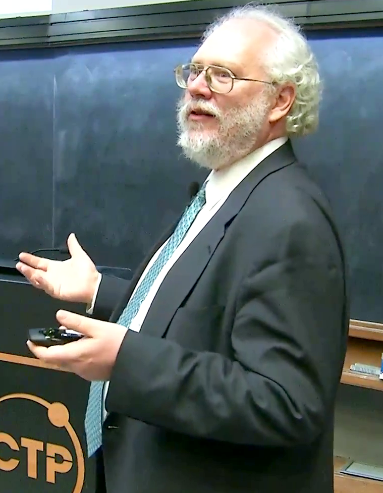
Peter Shor
Ref:
Wikipedia
Two Motivations, One Physical Thesis
| Motivation | Question | Lesson |
|---|---|---|
| Feynman | How can we efficiently simulate quantum nature? | Use a quantum system as the simulator. |
| Shor | Can quantum dynamics accelerate a non-simulation task? | The physical model can change computational complexity. |
| Shared thesis | Can computation be separated from its physical laws? | Computation is physical. |
One-Minute Contrast
Complete both sentences: “Feynman motivates quantum computing because …”; “Shor changes the discussion because …”.
What Does a Qubit Actually Add?
A qubit has state (\alpha|0\rangle+\beta|1\rangle), but measurement does not reveal both amplitudes. The useful resource is not “reading all answers at once.” Algorithms arrange relative phases so that later evolution converts them into enhanced or suppressed outcome probabilities.
\[|0\rangle\xrightarrow{H}\frac{|0\rangle+|1\rangle}{\sqrt2}\xrightarrow{Z}\frac{|0\rangle-|1\rangle}{\sqrt2}\xrightarrow{H}|1\rangle.\]
\[\boxed{\text{superposition}+\text{phase control}+\text{interference}+\text{measurement}.}\]
Transition: Can ordinary irreversible logic be inserted directly into this coherent evolution?
Exponential State Description: What It Does and Does Not Prove
An arbitrary \(n\)-qubit vector has \(2^n\) amplitudes, but amplitude counting alone is not a proof of computational speedup. Many physically important states have symmetry, low entanglement, stabilizer structure, tensor-network descriptions, or other compressed representations.
The defensible conclusion is narrower:
\[\text{generic quantum state space is exponentially large,}\]
so a classical simulation method must exploit structure or pay a large representation cost. Quantum advantage arises only when state preparation, evolution, and useful measurement are all efficient while classical alternatives remain costly.
Digital Quantum Simulation
For \(H=\sum_j H_j\), time evolution may be approximated by product formulas. A first-order Trotter step is
\[e^{-iHt}\approx\left(\prod_j e^{-iH_jt/r}\right)^r.\]
Increasing \(r\) reduces approximation error but increases circuit depth. A complete resource analysis must include Hamiltonian representation, product-formula or block-encoding error, gate synthesis, qubit mapping, and fault-tolerance overhead.
Feynman's idea therefore leads directly to hardware questions: which interactions are native, which must be compiled, and whether coherence lasts through the required simulation time.
Phase Becomes Information Only through Interference
The states
\[|+\rangle=\frac{|0\rangle+|1\rangle}{\sqrt2},\qquad | -\rangle=\frac{|0\rangle-|1\rangle}{\sqrt2}\]
produce identical \(Z\)-basis statistics, yet \(H|+\rangle=|0\rangle\) and \(H|-\rangle=|1\rangle\). Relative phase is operationally meaningful because a later basis change converts it to population.
For many qubits, algorithms arrange phases globally so unwanted computational paths interfere destructively. Measurement samples the resulting distribution; it does not expose the state vector directly.
Shor's Algorithm as a Pipeline
- Reduce factoring \(N\) to finding the order \(r\) of \(a\bmod N\).
- Create a coherent superposition of exponents.
- Compute modular exponentiation reversibly.
- Use phase estimation / the quantum Fourier transform to extract information about \(r\).
- Apply continued fractions and classical number theory to recover factors.
The quantum computer does not simply “try every factor.” Its advantage comes from encoding periodic structure into phase and extracting that structure through interference.
The modular-arithmetic circuit, not the textbook QFT diagram alone, dominates much of the logical resource cost.
From Algorithmic Speedup to Practical Advantage
Keep four claims separate:
- Asymptotic algorithmic result: scaling in an ideal model.
- Logical resource estimate: encoded qubits and logical operations.
- Fault-tolerant implementation: code distance, factories, decoding, and cycles.
- System advantage: wall-clock time, energy, cost, reliability, and comparison with the best classical method.
A compelling algorithm may still be beyond current hardware; a modest subroutine may become useful earlier if it matches native operations and admits verification.
Phase Estimation as the Reusable Core of Shor
Suppose \(U|u\rangle=e^{2\pi i\phi}|u\rangle\). Quantum phase estimation transfers information about \(\phi\) into a control register by controlled powers \(U^{2^k}\), then applies an inverse quantum Fourier transform:
\[|0\rangle^{\otimes t}|u\rangle\rightarrow\sum_{j=0}^{2^t-1}e^{2\pi i j\phi}|j\rangle|u\rangle\rightarrow|\widetilde{\phi}\rangle|u\rangle.\]
The circuit illustrates the full quantum-algorithm grammar: superposition creates paths, controlled evolution writes phase, interference converts phase into population, and measurement produces a finite-precision estimate. In Shor, \(U\) is related to modular multiplication; implementing its controlled powers reversibly is the dominant problem-specific work.
Iterative phase estimation can trade coherent qubits for repeated measurements and classical feed-forward, reminding us that equivalent algorithms may distribute resources differently.
Q4. Why Must Reversible Computation Meet Quantum Dynamics?
From Boolean Functions to Unitary and Hamiltonian Evolution
The Collision: Many-to-One Logic versus One-to-One Evolution
AND maps four input pairs to one output bit. Three inputs share the same output:
\[(0,0),(0,1),(1,0)\mapsto0,\qquad(1,1)\mapsto1.\]
A closed quantum system evolves unitarily. Since (U^\dagger U=I), inner products are preserved:
\[\langle U\psi|U\phi\rangle=\langle\psi|\phi\rangle.\]
Two distinguishable inputs therefore cannot be mapped to the same complete output state by an ordinary unitary operation.
Reversible Embedding
An irreversible function is embedded in a larger one-to-one map:
\[U_f:|x\rangle|y\rangle\mapsto|x\rangle|y\oplus f(x)\rangle.\]
For AND, the Toffoli transformation is
\[|a,b,y\rangle\mapsto|a,b,y\oplus ab\rangle.\]
The original inputs are retained, and the target is toggled rather than overwritten. Reversibility costs resources: extra registers, gates, routing, and time.
Board Task
Write all eight input-output rows and verify that the mapping is a permutation.
Bennett: Compute, Copy, Uncompute
- Compute: retain intermediate results rather than overwrite them.
- Copy: copy a classical-basis result into a clean output register.
- Uncompute: run the reversible circuit backward to return temporary registers to a standard state.
Uncomputation is essential in quantum algorithms because unused garbage may remain entangled with the desired output and destroy later interference.
Landauer's principle supplies the thermodynamic warning: logically irreversible reset has a physical entropy cost. Logical reversibility does not guarantee zero dissipation, but information loss cannot be treated as an abstract bookkeeping operation.
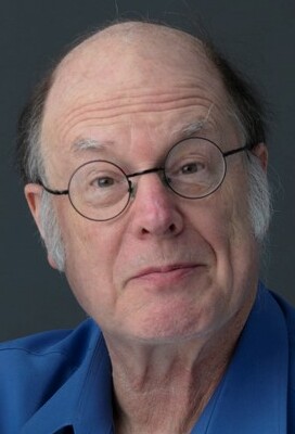
Charles H. Bennett
Ref:
Wikimedia Commons
▲
Ref:
https://commons.wikimedia.org/wiki/File:Dr._Charles_Bennett_IBM_Fellow_(cropped).jpg
From Reversible Logic to Physical Evolution
A reversible classical gate permutes computational-basis states. A quantum gate extends the transformation linearly to arbitrary superpositions. A device must then generate that unitary through a Hamiltonian:
\[i\hbar\frac{d}{dt}|\psi(t)\rangle=H(t)|\psi(t)\rangle,\]
\[U(T)=\mathcal T\exp\!\left[-\frac{i}{\hbar}\int_0^T H(t)\,dt\right].\]
\[\boxed{\text{Boolean function}\rightarrow\text{reversible embedding}\rightarrow\text{unitary}\rightarrow H(t).}\]
Break · Keep This Bridge on the Board
\[\text{mechanized rules}\rightarrow\text{universal computation}\rightarrow\text{quantum motivation}\rightarrow\text{reversible embedding}\rightarrow\text{unitary dynamics}.\]
Return with one question: if unitary gates are only one way to organize quantum evolution, where else can the “program” be stored?
Landauer Bound with Numbers
Resetting an unbiased bit reduces its information entropy by \(k_B\ln2\). In an ideal quasistatic process, the environment must receive at least
\[Q_{\min}=k_BT\ln2.\]
At \(300\,\mathrm K\), \(Q_{\min}\approx2.87\times10^{-21}\,\mathrm J\). Formally, at \(10\,\mathrm{mK}\), it is approximately \(9.57\times10^{-26}\,\mathrm J\).
This is not an estimate of total computer power. Refrigeration, control electronics, attenuation, amplification, finite-time switching, and error correction dominate real systems. Landauer supplies a lower bound for logically irreversible reset under stated assumptions.
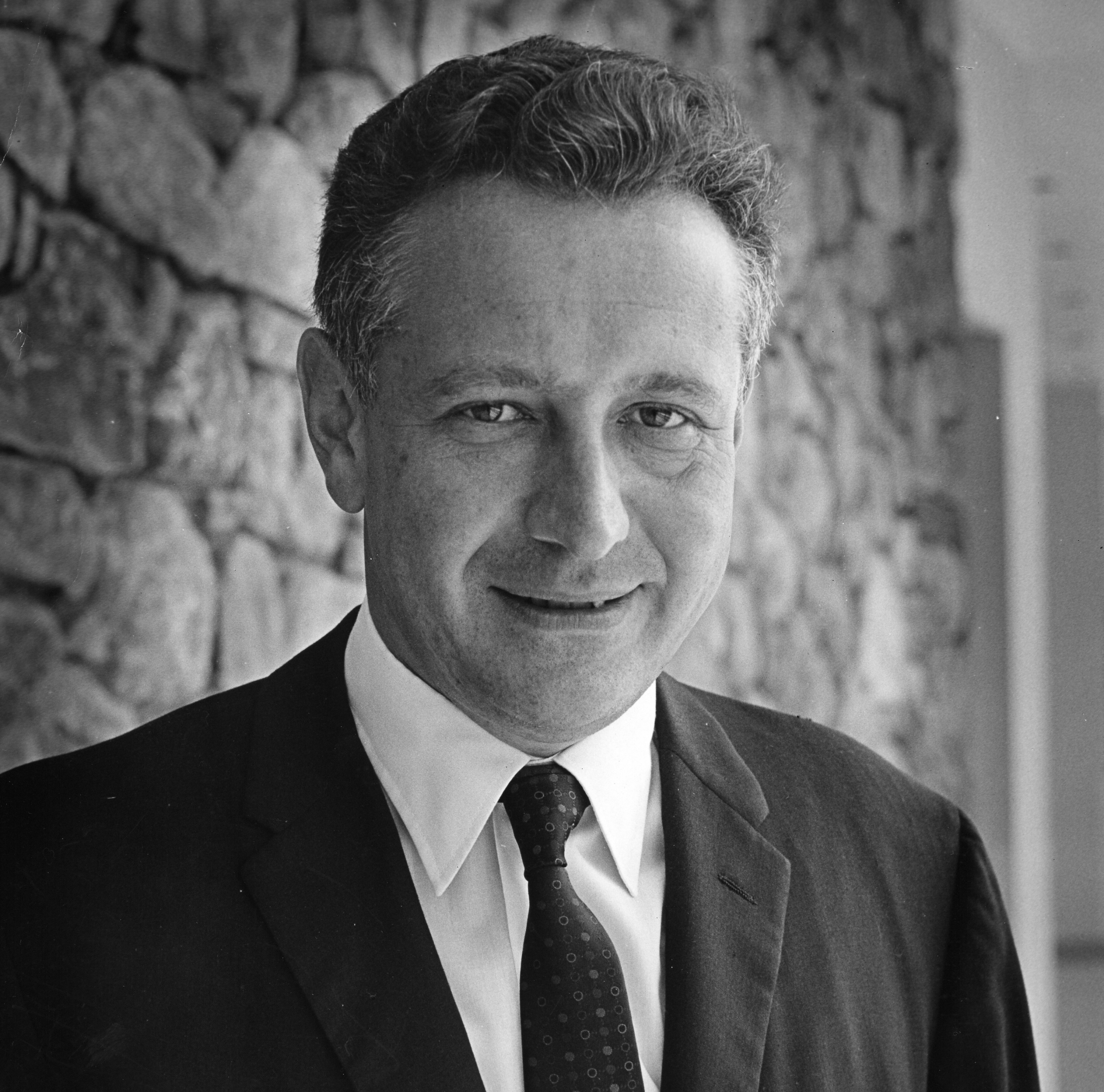
Rolf Landauer
Ref:
Wikimedia Commons
▲
Ref:
https://commons.wikimedia.org/wiki/File:Rolf_Landauer.jpg
Logical and Thermodynamic Reversibility Differ
| Logical reversibility | Thermodynamic reversibility |
|---|---|
| Property of an input-output map | Property of a physical trajectory |
| Input is recoverable from output | Entropy production can approach zero |
| Toffoli is reversible | A fast noisy Toffoli may dissipate strongly |
| Does not specify timing or damping | Depends on protocol, bath, and rate |
Likewise, unitary evolution of a closed system does not imply that an entire quantum computer—including initialization, measurement, reset, and feedback—is dissipation free.
Density Matrices Make the Boundary Visible
A closed system follows \(\rho\mapsto U\rho U^\dagger\). A general physical quantum operation on a subsystem is a completely positive trace-preserving map:
\[\mathcal E(\rho)=\sum_k E_k\rho E_k^\dagger,\qquad\sum_kE_k^\dagger E_k=I.\]
Projective measurement with outcome \(m\) has probability and conditional state
\[p_m=\mathrm{Tr}(P_m\rho),\qquad \rho_m=\frac{P_m\rho P_m}{p_m}.\]
The enlarged system-plus-apparatus may evolve unitarily, while conditioning on a classical record makes the subsystem description non-unitary.
Clean Oracle Worked Example
Suppose \(g=a\oplus b\) is temporary and \(f=g\land c\) is required. A reversible implementation:
- Compute \(g\) into ancilla \(r\): \(r\leftarrow r\oplus a\oplus b\).
- Compute \(f\) into output \(y\): \(y\leftarrow y\oplus rc\).
- Reverse the first step to restore \(r=0\).
If step 3 is omitted while inputs are in superposition, \(r\) remains correlated with the computational paths. Ignoring it is equivalent to discarding which-path information and can suppress later interference.
From Addition to Reversible Arithmetic
An irreversible full adder retains only sum and carry, discarding part of the input history. A reversible arithmetic circuit instead preserves inputs or writes results into clean targets. For an \(n\)-bit register, even a conceptually simple addition requires choices about carry propagation, ancilla allocation, uncomputation, and connectivity.
A ripple-carry design uses few ancillas but has depth proportional to \(n\). Carry-lookahead reduces asymptotic depth by generating and combining carry information in parallel, but uses more workspace and nonlocal interactions. Fault-tolerant compilation adds another accounting layer because Toffoli or controlled rotations expand into costly logical primitives.
Design Decision
If qubits are scarce but coherence time is generous, which design pressure dominates? How does the answer change when logical depth, rather than qubit count, is the limiting resource?
Toffoli Is Not a Hardware Button
The notation CCX hides a three-qubit unitary. A platform with only one-qubit rotations and a native two-qubit entangler must synthesize it. Exact and relative-phase Toffoli constructions may agree on computational-basis outputs while differing on phases.
If the output is measured immediately in the computational basis, some phase freedom may be harmless. If the operation appears inside amplitude amplification or uncomputation, an untracked relative phase changes later interference. The compiler therefore needs semantic context, not just a truth table.
After synthesis, routing may insert SWAP operations because the three logical qubits are not adjacent. Scheduling must avoid frequency collisions and simultaneous-control crosstalk. Pulse calibration then determines the actual unitary, and tomography or randomized protocols supply evidence that the intended operation was reached.
Q5. Must Quantum Computation Be Expressed as a Sequence of Gates?
Circuits, Measurements, and Hamiltonian Paths
Gate-Based Computation: Program as a Circuit
\[|\psi_{\mathrm{out}}\rangle=G_mG_{m-1}\cdots G_1|\psi_{\mathrm{in}}\rangle.\]
The program is a sequence of discrete logical operations. A universal gate set approximates arbitrary target unitaries to a chosen accuracy. It does not imply that all gates cost the same or that hardware provides ideal gate symbols directly.
Primary resources: coherent qubits, accurate one- and two-qubit operations, connectivity, depth, mid-circuit measurement when required, and classical control.
Measurement-Based Computation: Program as an Adaptive Measurement Pattern
Prepare a highly entangled resource state, such as a cluster state, then compute through local measurements:
\[\text{resource state}\rightarrow\text{measurement basis and order}\rightarrow\text{classical feed-forward}\rightarrow\text{logical output}.\]
Measurements consume the resource state and teleport logical information through it. Earlier outcomes determine later measurement bases.
Measurement-based computation can implement logical gates and can be translated to a circuit, but it is not physically “just a gate circuit.” Its native execution primitives are entangled-state preparation, measurement, and feed-forward—especially important in photonic platforms.
Adiabatic Computation: Program as a Hamiltonian Path
\[H(s)=(1-s)H_{\mathrm{initial}}+sH_{\mathrm{problem}},\qquad 0\le s\le1.\]
The system begins near an easily prepared ground state. The Hamiltonian changes according to (s(t)); sufficiently slow evolution relative to the relevant spectral structure keeps the state near the desired path.
The program is encoded in (H_{\mathrm{problem}}), the interpolation path, and the schedule. Key costs include embedding, the minimum gap, thermal excitation, control error, and total evolution time.
Two Ways to Program Quantum Evolution
Gate-Based / Circuit Model
Program = an ordered circuit of discrete operations
- Algorithms such as Shor, Grover, and phase estimation
- Digital quantum simulation
- Discrete gates, measurements, and classical feed-forward
Adiabatic Evolution & Quantum Annealing
Program = a Hamiltonian, an interpolation path, and a schedule
- Optimization and ground-state search
- Problem encoded in a Hamiltonian, often Ising/QUBO
- Continuous schedule; minimum gap, noise, and temperature matter
Concept reference: Chen et al. · energy-landscape figure (diagram redrawn)
Related, not identical: adiabatic quantum computation is a computational model; quantum annealing is a practical search strategy; an Ising Hamiltonian is a common problem encoding.
Gate-Based vs. Adiabatic Quantum Computing
Gate-Based / Circuit Model
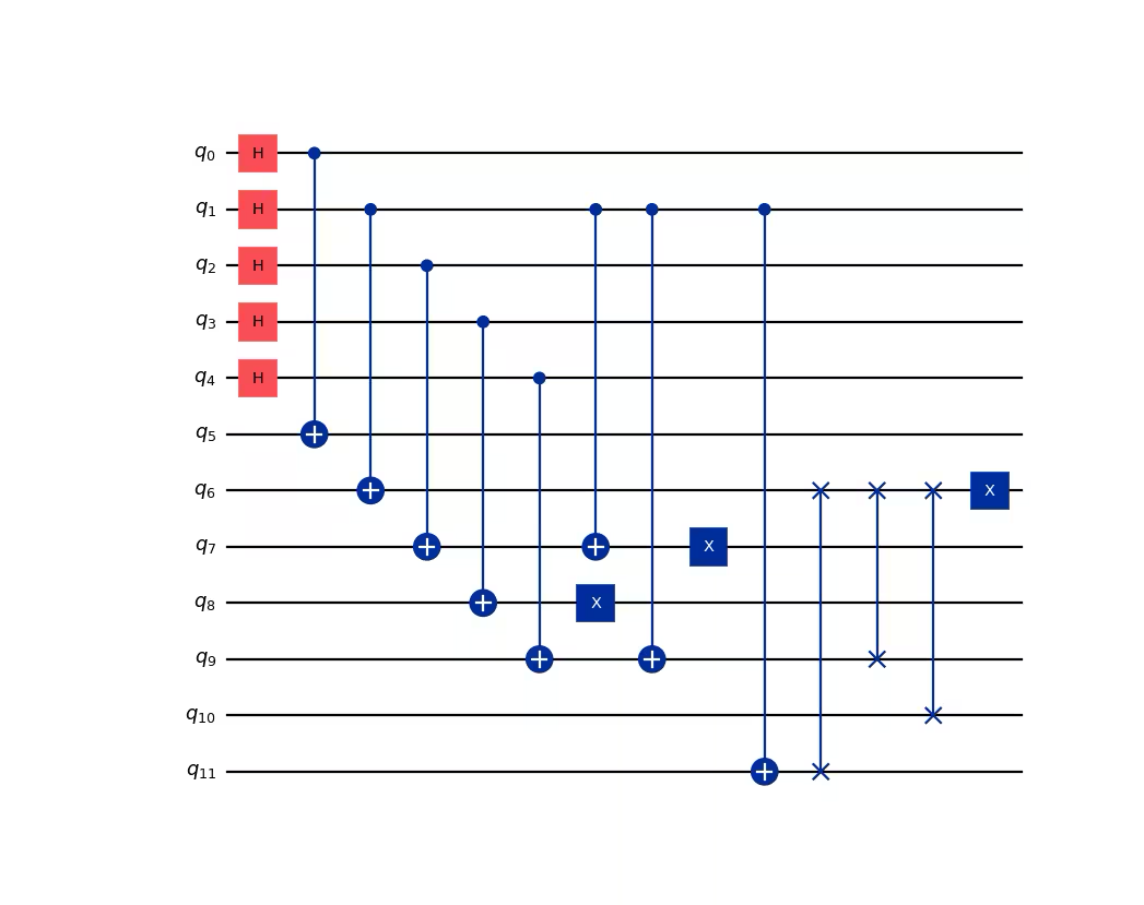








Adiabatic Evolution / Quantum Annealing
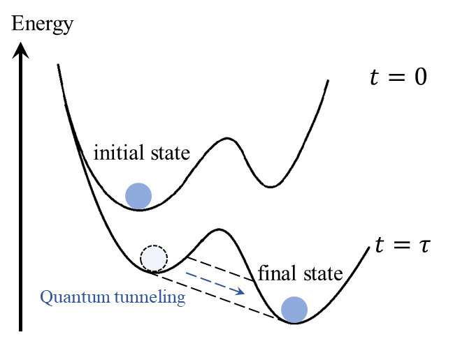

Equivalent Power Does Not Mean Equivalent Engineering
| Question | Gate-based | Measurement-based | Adiabatic |
|---|---|---|---|
| Where is the program? | Gate sequence | Graph state and measurement pattern | Hamiltonian path and schedule |
| Primary primitive | Unitary gate | Adaptive local measurement | Continuous evolution |
| Key resource | Coherent controllable qubits | Entangled resource state | Ground-state path and gap |
| Typical failure | Gate error, crosstalk, decoherence | Loss, wrong basis, feed-forward latency | Excitation, small gap, thermal error |
Architecture Activity
For each model, identify: (1) representation, (2) memory/resource state, (3) allowed operation, (4) control flow, and (5) input/output. Then select the interface most likely to dominate experimental difficulty.
Takeaway
Computational equivalence is a statement at the logical-model layer. Preparation, coherence, connectivity, feedback bandwidth, calibration, and readout can differ completely.
Gate Universality and Approximation
A continuous family of unitaries cannot be represented exactly by arbitrary finite strings from a finite discrete gate set. Universality normally means approximation to accuracy \(\epsilon\). The compiler must choose a decomposition and track accumulated error.
On superconducting hardware, a native basis might include virtual \(R_z(\theta)\), calibrated \(X_{\pi/2}\), and an entangling \(CZ\) or echoed cross-resonance operation. The logical symbol \(H\), CNOT, or Toffoli expands into these primitives.
Semantic equivalence on basis states is weaker than full unitary equivalence: relative phases matter whenever the result participates in later interference.
Measurement-Based Computation through Teleportation
In a cluster state, measuring one qubit can teleport the logical state to a neighbor while applying a basis-dependent rotation. Random outcomes introduce known Pauli byproducts. Later measurement angles are adapted so computation remains deterministic at the logical level.
\[|\psi\rangle\xrightarrow[\text{entangle}]{CZ}\text{cluster}\xrightarrow[\text{angle }\alpha]{\text{measure}}X^mHR_z(\alpha)|\psi\rangle.\]
The bit \(m\) is random but known. Classical feed-forward updates the interpretation or the next basis. The “program” is therefore distributed across the graph, measurement angles, ordering, and classical side processing.
Adiabatic Condition and the Minimum Gap
Let \(s=t/T\). A schematic adiabatic requirement has the form
\[T\gg\max_s\frac{|\langle1(s)|\partial_sH|0(s)\rangle|}{\Delta(s)^2},\qquad \Delta(s)=E_1(s)-E_0(s).\]
The exact bound depends on smoothness and theorem assumptions, but the engineering lesson is stable: a small minimum gap can require long evolution, while finite temperature and noise can excite the system away from the desired state.
Equivalent computational power to the circuit model does not imply equal physical runtime or identical robustness.
One Problem, Three Program Locations
| Layer | Circuit | Measurement based | Adiabatic |
|---|---|---|---|
| Initial resource | Register state | Entangled graph state | Ground state of \(H_0\) |
| Program | Ordered gates | Angles, order, feed-forward | \(H(s)\) and \(s(t)\) |
| Clock | Gate scheduler | Measurement dependencies | Continuous schedule |
| Readout | Bit-string samples | Measurement record plus Pauli frame | Final energy/configuration samples |
The correct hardware question is not “which diagram looks simpler?” but “which expensive resource has been moved or hidden?”
Gate Teleportation Connects Circuit and Measurement Models
Quantum teleportation shows how entanglement, measurement, and classical communication can reproduce a logical state transfer without directly moving the carrier. Gate teleportation extends the idea: prepare a resource state containing the desired operation, perform joint or local measurements, and interpret the output with outcome-dependent Pauli corrections.
This explains why measurement-based computation can be logically translated into gates while remaining physically distinct. In a circuit description, the correction may appear as a conditional \(X\) or \(Z\). In hardware, it may be implemented as a virtual Pauli-frame update rather than a physical pulse. In photonics, fast feed-forward, detector efficiency, indistinguishability, and resource-state generation become architectural bottlenecks.
“Equivalent to a circuit” is a theorem about achievable logical transformations; it is not permission to erase the preparation and feed-forward costs.
Avoided Crossing and Adiabatic Runtime
Consider the two-level Hamiltonian
\[H(s)=\frac{1}{2}\left[v(s-s_0)\sigma_z+\Delta_{\min}\sigma_x\right].\]
The instantaneous gap is \(\Delta(s)=\sqrt{v^2(s-s_0)^2+\Delta_{\min}^2}\). Near \(s_0\), the eigenstates change most rapidly and the gap is smallest. A uniform schedule may waste time far from the avoided crossing and move too rapidly near it; a local adiabatic schedule slows where the gap is small.
Increasing total runtime can suppress diabatic transitions but creates more opportunity for thermal excitation, dephasing, and low-frequency control drift. “Go slowly” is therefore not an unlimited prescription in an open device.
Q6. How Does a Computational Model Become Hardware—and What Ultimately Limits It?
From Logical Instructions to Physical and Gravitational Bounds
The Cross-Layer Execution Chain
For a superconducting gate-based processor:
\[\boxed{\text{problem}\rightarrow\text{algorithm}\rightarrow\text{logical circuit}\rightarrow\text{native gates}\rightarrow H(t)\rightarrow\text{waveform}\rightarrow\text{measurement record}.}\]
Each arrow introduces new freedoms and new failure modes. An ideal gate does not specify frequency, coupling, pulse envelope, duration, leakage, crosstalk, readout assignment, or recalibration policy.
The Real Output Is Data, Not a Ket
Control electronics translate a schedule into microwave and flux waveforms. The device produces an analog response, which is amplified, down-converted, integrated, classified, and accumulated over repeated shots.
\[\text{AWG file}\rightarrow\text{cryogenic signal}\rightarrow\text{qubit evolution}\rightarrow\text{resonator response}\rightarrow\text{IQ point}\rightarrow\text{bit-string counts}.\]
Validation therefore requires more than agreement with one truth table: phase-sensitive tests, calibration baselines, error bars, drift monitoring, and a model that links observed failure to a specific layer.
A Validation Ladder
- Characterize levels, transition frequencies, anharmonicity, (T_1), (T_2), and readout.
- Calibrate single-qubit amplitude, phase, detuning, and leakage control.
- Calibrate two-qubit interactions and relevant connectivity edges.
- Test simultaneous operations, crosstalk, and calibration drift.
- Execute the compiled circuit and compare with a complete error budget.
Fault Localization
If an AND/Toffoli experiment returns the wrong bit string, name one possible failure at the semantic, compilation, control, device, and measurement layers.
Computation Approaching the Limits of Physics
| Scale | Constraint | Question |
|---|---|---|
| Engineering | Noise, fabrication, cooling, control | Can the operation be repeated reliably? |
| Quantum | Measurement, coherence, quantum speed limits | How fast can distinguishable states evolve? |
| Thermodynamic | Entropy production and heat removal | What is the cost of reset and error correction? |
| Relativistic | Finite signal-propagation speed | How quickly can a large machine coordinate? |
| Gravitational | Finite energy and information density | When can gravity no longer be neglected? |
The Ultimate Calculator
If more memory and faster operations require physical degrees of freedom, energy, communication, and error removal, then packing unlimited computation into a finite region is impossible. At sufficiently high energy density, gravity enters the design problem and gravitational collapse becomes relevant.
Final question: If we try to build the ultimate calculator inside a finite volume, will adding more memory and computational energy eventually turn the calculator into a black hole?
This is a boundary question, not the assertion that every ultimate computer literally is a black hole. Its purpose is to show that a complete theory of computation eventually brings information, quantum mechanics, thermodynamics, relativity, and gravity into the same conversation.
From Circuit Elements to an Artificial Atom
A transmon is approximately described by
\[H=4E_C(\hat n-n_g)^2-E_J\cos\hat\phi.\]
The Josephson cosine supplies nonlinearity; the capacitor supplies charging energy. After quantization and truncation, the lowest levels form a qubit only approximately. The higher levels remain physically present, producing anharmonicity and leakage constraints.
A Josephson junction is therefore not a natural “gate.” It supplies a Hamiltonian from which levels, transitions, couplings, drive operators, and readout channels must be engineered.
A Microwave Pulse as a Rotation
Near resonance and in a rotating-wave description, a driven qubit may have
\[H_{\mathrm{rot}}(t)=\frac{\hbar}{2}\left[\Delta\sigma_z+\Omega_x(t)\sigma_x+\Omega_y(t)\sigma_y\right].\]
On resonance, pulse area sets the rotation angle:
\[\theta=\int_0^T\Omega(t)\,dt.\]
The abstract operation \(R_x(\pi/2)\) thus becomes a calibrated amplitude, phase, envelope, carrier frequency, and duration. Detuning, distortion, finite anharmonicity, and crosstalk make the realized operation differ from the target.
Dispersive Readout Produces an Inference Problem
In the dispersive regime, qubit state shifts a resonator response. A measurement chain produces noisy IQ trajectories, not direct labels:
\[V(t)\rightarrow z=\int w(t)V(t)dt\rightarrow(I,Q)\rightarrow\widehat{b}.\]
Assignment error includes overlap of conditional IQ distributions, state relaxation during measurement, preparation error, amplifier noise, and classifier bias. Multi-qubit readout additionally introduces correlated errors and measurement crosstalk.
Consequently, “the answer is a ket” belongs to the model layer; the laboratory answer is a statistical dataset plus an inference procedure.
A Cross-Layer Error Budget
| Layer | Representative quantity | Diagnostic |
|---|---|---|
| Algorithm | Approximation / success probability | Ideal simulation |
| Compilation | Depth, routing, synthesis error | Equivalence and resource checks |
| Control | Over-rotation, phase, leakage | Rabi, Ramsey, randomized benchmarking |
| Device | \(T_1,T_2\), coupling, drift | Spectroscopy and time-domain characterization |
| Measurement | Assignment matrix, correlated error | Prepared-state calibration |
Multiplying nominal component fidelities is only a first estimate; coherent error, correlations, drift, and context dependence can invalidate independent-error assumptions.
Speed, Energy, Information, and Gravity
Several different limits should not be collapsed into one slogan:
- Landauer: entropy cost of logically irreversible reset.
- Quantum speed limits: energy and state distinguishability constrain evolution time.
- Relativity: control and communication cannot propagate instantaneously.
- Finite-density bounds: finite energy and size constrain distinguishable information.
- Gravitational collapse: concentrating sufficient energy inside a small radius changes spacetime and can form a horizon.
These limits arise under different assumptions and are not a single formula for computer performance. Together they show why ultimate computation becomes a problem for fundamental physics.
Black Hole: Computer, Memory Bound, or Boundary of Description?
For mass \(M\), the Schwarzschild radius is \(r_s=2GM/c^2\). If increasing a finite machine's energy pushes its physical size toward the corresponding gravitational radius, a nongravitational circuit model is no longer self-consistent.
The pedagogical conclusion is deliberately conditional:
\[\text{more density}\rightarrow\text{gravity matters}\not\Rightarrow\text{every best computer is literally a black hole}.\]
Open questions connect black-hole entropy, information recovery, quantum error correction, and spacetime. They are a powerful finale precisely because no single settled engineering blueprint follows from them.
Extended Synthesis Matrix
| Question | Abstract object | Physical object | Hidden cost |
|---|---|---|---|
| Q1 Mechanization | Rule | State-transition device | Timing and reliability |
| Q2 Computability | Machine model | Programmable architecture | Resource scaling |
| Q3 Quantum motivation | Amplitude algorithm | Coherent many-body system | Preparation and verification |
| Q4 Reversibility | Unitary embedding | Controlled Hamiltonian | Ancilla and uncomputation |
| Q5 Models | Equivalent computation | Different native primitives | Resource relocation |
| Q6 Hardware | Ideal operation | Waveforms and records | Error, heat, space, time |
Turning a Pulse Error into a Circuit Error
An intended \(X_{\pi/2}\) pulse with fractional amplitude error \(\varepsilon\) implements \(R_x[(1+\varepsilon)\pi/2]\). The coherent over-rotation accumulates systematically if repeated with the same phase. A sequence of \(m\) identical errors can produce an angle error proportional to \(m\varepsilon\), rather than behaving like independent random noise.
This is why average gate fidelity alone cannot predict every circuit. Calibration sequences, randomized benchmarking, cycle benchmarking, and application-level tests probe different error combinations. Echoes or randomized compiling can convert some coherent accumulation into a more stochastic effective channel, but may increase duration or pulse count.
An error model is itself an interface: algorithmic estimates depend on whether hardware errors are local, Markovian, biased, correlated, drifting, or leakage-producing.
Measurement, Reset, and the Computation Cycle
A useful quantum computer repeatedly performs a cycle that is not globally described by one closed-system circuit:
\[\text{initialize}\rightarrow\text{coherent control}\rightarrow\text{measure}\rightarrow\text{classical inference}\rightarrow\text{feedback/reset}.\]
Passive reset waits several \(T_1\) times; active reset measures and conditionally drives; engineered dissipation transfers entropy to an auxiliary mode or bath. Each method trades latency, residual excitation, hardware complexity, and calibration burden.
Fault-tolerant error correction intensifies this interface. Syndrome ancillas must be prepared, entangled, measured, decoded, and reset repeatedly while logical data remain coherent. Classical processing is not outside the quantum computer: its latency and reliability enter the quantum error budget.
The Ultimate Calculator as a Consistency Test
Imagine specifying a computer only by an operation count. Physics immediately demands missing parameters: available energy, operating temperature, physical volume, communication distance, allowed error, and total time. Increasing one resource can worsen another. More energy can permit faster evolution but complicates cooling; denser packing shortens wires but strengthens unwanted interactions; stronger error correction consumes more operations and entropy-removal capacity.
At ordinary scales these are engineering trade-offs. At extreme scales, the assumptions behind the circuit model themselves fail: clocks cannot synchronize instantaneously, energy gravitates, and a finite region cannot hold arbitrarily many distinguishable physical states. The black-hole finale is therefore not decorative science fiction. It is a stress test of the claim that computation can be specified independently of the universe that performs it.
A complete account of achievable computation must be consistent with quantum theory, thermodynamics, relativity, and gravity—even when no single “ultimate computer” construction saturates every bound simultaneously.
Q7. Can a Machine Completely Describe, Predict, and Reproduce Itself?
Gödel, Turing, Self-Reference, and Self-Reproducing Automata
When a Formal System Talks about Itself
Mechanization turns expressions, proofs, and programs into finite symbolic objects. Once those objects can themselves be encoded as numbers or strings, a system may receive a description of its own rules—or even its own description—as input.
\[\boxed{\text{description of an object}\longrightarrow\text{data manipulated inside the same formal system}.}\]
This enables compilers, interpreters, universal machines, and self-reproducing systems. It also enables diagonal constructions that expose limits: a statement or program can be built to react to what the system says about that very statement or program.
Self-reference is not automatically a contradiction. The result depends on how the self-referential object is constructed and which consistency or decision assumptions are imposed.
Gödel Numbering: Syntax Becomes Arithmetic
Gödel's key move was to encode symbols, formulas, and sequences of formulas by integers. Relations such as “\(x\) is a valid proof of statement \(y\)” could then be represented arithmetically inside a sufficiently expressive formal system.
This makes metamathematical claims—claims about formulas and proofs—available as statements within arithmetic itself. A diagonal construction produces a sentence whose content is, schematically:
\[G\;\longleftrightarrow\;\text{“\(G\) is not provable in this system.”}\]
The construction is more precise than the informal liar paradox. It refers to formal provability through encoded syntax, not directly to an undefined notion of truth.
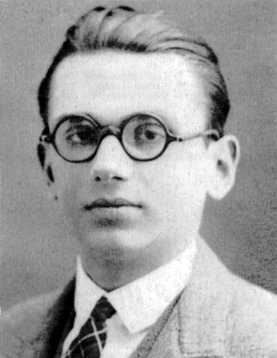
Kurt Gödel, 1924–1927
Ref:
Wikimedia Commons
▲
Ref:
https://commons.wikimedia.org/wiki/File:1925_kurt_g%C3%B6del.png
What Gödel's Incompleteness Theorems Actually Say
For a consistent, effectively axiomatized formal system strong enough to express elementary arithmetic:
- First incompleteness theorem: there are arithmetic statements that the system cannot decide; under the relevant assumptions, its Gödel sentence is not provable within the system.
- Second incompleteness theorem: such a system cannot prove its own consistency using only its internal resources, assuming it is in fact consistent.
Gödel did not prove that mathematics is futile, that every true statement is unprovable, or that human minds automatically transcend machines. The result identifies a limit on the simultaneous goals of effective axiomatization, sufficient expressive power, consistency, and completeness.
Turing Turns the Limit into a Machine Question
Suppose a program \(\mathrm{HALT}(P,x)\) correctly decides whether every program \(P\) eventually halts on input \(x\). Construct a new program \(D(P)\):
- Run \(\mathrm{HALT}(P,P)\).
- If it predicts “halts,” loop forever.
- If it predicts “does not halt,” halt immediately.
Now ask what \(D(D)\) does:
\[D(D)\text{ halts}\iff D(D)\text{ does not halt}.\]
The contradiction shows that no single algorithm decides halting correctly for every possible program-input pair.
Gödel and Turing Share a Diagonal Structure
| Gödel | Turing | Shared structure |
|---|---|---|
| Encode formulas and proofs as numbers | Encode programs and inputs as strings | Descriptions become objects within the system |
| Construct a sentence about its own provability | Run a program on its own description | Self-application |
| Derive incompleteness from a completeness assumption | Derive undecidability from a universal decider assumption | Diagonal reversal |
| Limit of formal proof | Limit of algorithmic decision | Universality does not imply omniscience |
These are related but not identical theorems. Gödel concerns formal axiomatic systems; Turing concerns algorithms and machine behavior. Their bridge is effective encoding and self-reference.
Von Neumann's Question: Can a Machine Construct Another Machine?
John von Neumann studied a different consequence of descriptions becoming data. A self-reproducing automaton must do more than copy material blindly: it must both interpret a description to construct a machine and copy that description into the offspring.
A schematic organization is:
- \(A\): a universal constructor that builds the machine described by \(I\);
- \(B\): a copier that duplicates description \(I\);
- \(C\): a controller coordinating construction and copying;
- \(I(A+B+C)\): the encoded description of the complete system.
\[(A+B+C)+I\longrightarrow[(A+B+C)+I]+[(A+B+C)+I].\]
The description plays two roles: executable instructions during construction and uninterpreted data during copying.
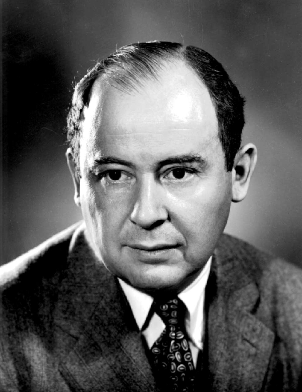
John von Neumann
Ref:
Wikimedia Commons
▲
Ref:
https://commons.wikimedia.org/wiki/File:JohnvonNeumann-LosAlamos.jpg
Self-Reproduction Is Not the Same as Self-Reference Paradox
Gödel and Turing use self-reference to challenge a proposed universal proof or decision procedure. Von Neumann uses self-description constructively: a description is interpreted once to build the machine and copied once to provide the offspring's description.
| Use of self-description | Purpose | Outcome |
|---|---|---|
| Gödel sentence | Refer to formal provability | Incompleteness |
| Diagonal halting program | Reverse a prediction about itself | Undecidability |
| Universal constructor | Interpret and copy a construction description | Self-reproduction |
The common foundation is encoded description. The logical operation performed on that description determines whether it yields a limit theorem, a universal simulator, or a reproducing system.
Cellular Automata: A Physics of Local Rules
Von Neumann developed his self-reproducing automaton in a cellular-automaton setting: a lattice of cells, each with a finite state, updated by the same local rule using nearby states.
\[s_i(t+1)=F\!\left(s_i(t),\{s_j(t):j\in N(i)\}\right).\]
This is a minimal model of mechanized physics:
- space is represented by a lattice;
- matter or information is represented by cell states;
- time advances in discrete updates;
- dynamics is local and uniform;
- complex global behavior emerges from simple repeated rules.
Von Neumann's original construction was not Conway's Game of Life; it used a more elaborate cellular-automaton rule designed for universal construction.
Conway's Game of Life: Simple Rules, Universal Behavior
In Conway's later two-dimensional Game of Life, each cell is alive or dead. Its next state depends on the number of live neighbors: survival with two or three, birth with three, and death otherwise.
From these local rules emerge still lifes, oscillators, moving gliders, information-carrying patterns, logic constructions, and universal computation. Life therefore illustrates a central lesson:
\[\boxed{\begin{gathered}\text{simple local law}+\text{structured initial condition}\\ \longrightarrow\text{open-ended computational behavior}\end{gathered}}\]
Self-reproducing patterns have also been engineered in Life, but they are later constructions, not von Neumann's original automaton. Life is valuable here as a visually accessible demonstration of emergence and computational universality.
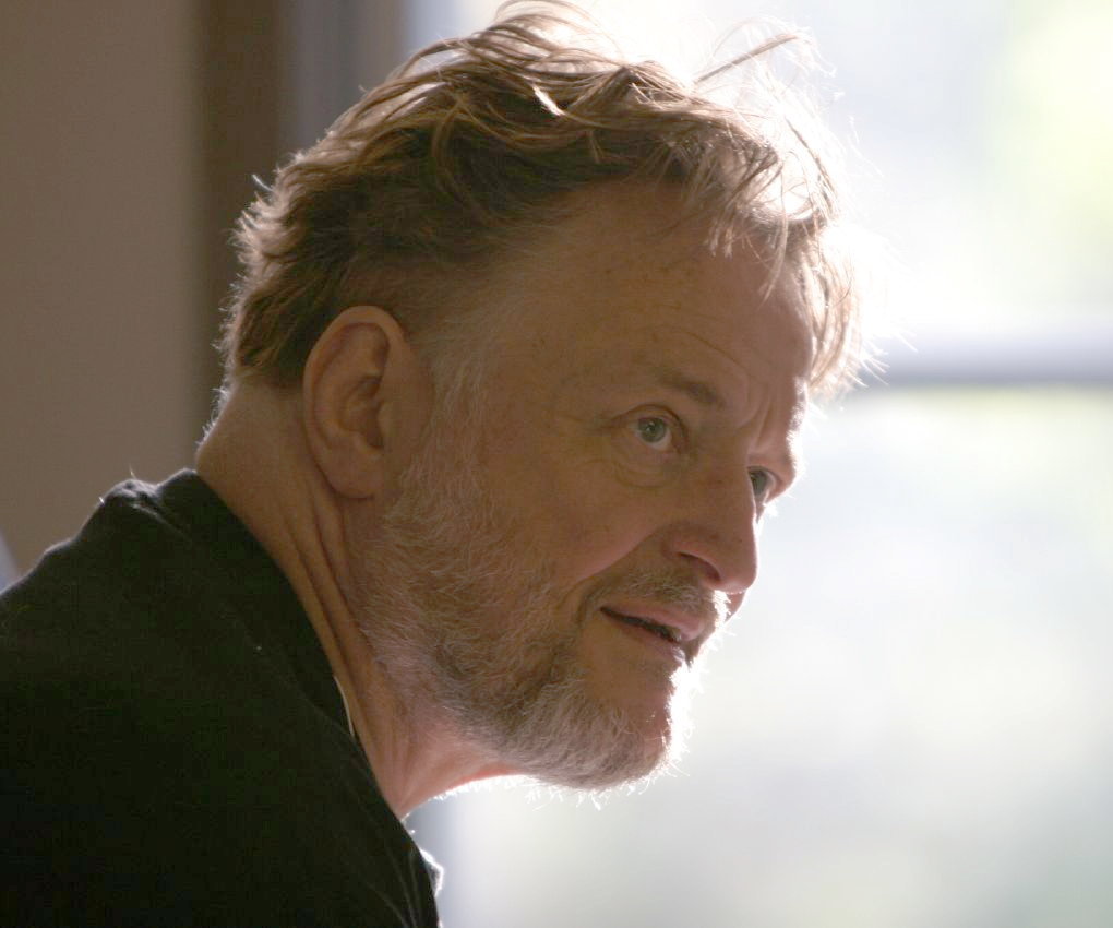
John Horton Conway, 2005
Ref:
Wikimedia Commons
▲
Ref:
https://commons.wikimedia.org/wiki/File:John_H_Conway_2005_(cropped).jpg
Final Synthesis: The Power and Limits of Encoded Description
The same conceptual invention appears throughout the lecture:
- A procedure is encoded so a machine can execute it.
- A machine description becomes input to a universal machine.
- A formal system encodes statements about proofs.
- A program receives its own description as data.
- A constructor interprets and copies the description of itself.
- A cellular automaton lets local physical rules generate universal computation.
Closing Question
Does self-description make a system all-knowing, or does it simultaneously enable universality, expose undecidable questions, and permit self-reproduction?
Exit Ticket: Reconstruct the Argument
In seven sentences—one per question—reconstruct how computation becomes a physical science with both constructive power and formal limits.
- What was mechanized?
- What boundary did computability establish?
- What did Feynman and Shor add?
- Why is reversible embedding necessary?
- Where can a quantum program live?
- Why must hardware and physical limits enter the theory?
- What does self-description enable, and what can it never decide universally?
Seven-Sentence Answer Guide
- Explicit symbolic procedures allow reasoning to be represented as mechanically executable state transformations.
- Computability identifies which procedures exist, while complexity measures their resource cost and universality describes programmable simulation.
- Feynman exposed the cost of simulating quantum nature, and Shor showed that quantum dynamics can change the complexity of a broader mathematical task.
- Closed quantum evolution is unitary, so irreversible functions must be embedded in larger reversible transformations.
- A quantum program may reside in a gate sequence, an adaptive measurement pattern, or a Hamiltonian path.
- Every model becomes a machine only through physical states, controls, measurements, and resources that ultimately obey thermodynamics, relativity, and gravity.
- Encoding descriptions as data enables universal simulation and self-reproduction, while diagonal self-reference reveals limits such as incompleteness and undecidability.
Core Reading: Foundations of Computation
- An Investigation of the Laws of ThoughtG. Boole (1854).Develops an algebraic treatment of logical reasoning.
- A Symbolic Analysis of Relay and Switching CircuitsC. E. Shannon (1938).Connects Boolean algebra to the analysis and synthesis of switching networks.
- Über formal unentscheidbare Sätze der Principia Mathematica und verwandter Systeme IK. Gödel (1931).Establishes incompleteness through arithmetization and diagonal self-reference.
- On Computable Numbers, with an Application to the EntscheidungsproblemA. M. Turing (1936).Formalizes mechanical computation and the universal machine.
- Theory of Self-Reproducing AutomataJ. von Neumann; edited by A. W. Burks (1966).Develops universal construction and self-reproduction in cellular automata.
- The Fantastic Combinations of John Conway's New Solitaire Game “Life”M. Gardner (1970).Introduces Conway's Game of Life and its emergent cellular-automaton behavior.
Further Reading: Quantum Motivation and Reversibility
- Simulating Physics with ComputersR. P. Feynman (1982).Motivates computers built from quantum-mechanical principles.
- Algorithms for Quantum Computation: Discrete Logarithms and FactoringP. W. Shor (1994).Shows polynomial-time quantum algorithms for factoring and discrete logarithms.
- Irreversibility and Heat Generation in the Computing ProcessR. Landauer (1961).Connects logical irreversibility to physical dissipation.
- Logical Reversibility of ComputationC. H. Bennett (1973).Develops reversible universal computation and uncomputation.
Further Reading: Quantum Models and Hardware
- A One-Way Quantum ComputerR. Raussendorf and H. J. Briegel (2001).Introduces measurement-based computation using entangled resource states.
- Quantum Computation by Adiabatic EvolutionE. Farhi et al. (2000).Formulates computation through continuous Hamiltonian evolution.
- A Quantum Engineer's Guide to Superconducting QubitsP. Krantz et al. (2019).Connects qubit physics, control, coherence, and readout.
Extended Foundations and Reference Modules
Optional Review and Self-Study Material
Advanced Throughline: Do Not Turn Week 1 into an Introduction to Quantum Information
This week assumes that students have already encountered kets, tensor products, and basic quantum gates. The class should not reteach every prerequisite; it should establish three descriptive layers:
- Computational semantics:inputs, outputs, computable functions, and complexity.
- Logical representation:reversible gates, unitary circuits, measurement, and classical feed-forward.
- Physical realization:the time-dependent Hamiltonian \(H(t)\), control pulses, and the measurement chain.
Landauer identifies the physical cost of “information erasure”; Bennett shows how a general computation can be rewritten as logically reversible by preserving history and applying uncomputation. The unitary evolution of quantum gates is therefore not merely a statement that “quantum mechanics is mysterious.” It is the intersection of information preservation, reversible dynamics, and implementable control.
\[\ket{\psi(t)}=\mathcal T\exp\!\left[-\frac{i}{\hbar}\int_0^t H(\tau)d\tau\right]\ket{\psi(0)}\]
Finally, compare the circuit model with the adiabatic/Hamiltonian model. They can be polynomially equivalent in computational power, but they expose different hardware control parameters, gaps, noise channels, and calibration problems.
Module 1: Classical Logic Gates and Boolean Computation
Classical Bits and Boolean Logic
Classical computation uses the bit as its most basic unit of information, and each bit can take only the value 0 or 1. At the hardware layer, these values usually correspond to high and low voltage, the presence or absence of charge, a magnetization direction, or another pair of stably distinguishable physical states. Boolean algebra allows complex logical operations to be decomposed into basic logic gates.
Core Concepts
- Bit: the smallest unit of classical information.
- Boolean algebra: represents logical false and true using 0 and 1.
- Truth table: tabulates the correspondence between a logic gate's inputs and outputs.
- Logic gate: a basic component that implements a Boolean operation.
Basic Logic Gates
| Gate | Input | Output | Functional Description |
|---|---|---|---|
| NOT | A | ¬A | Changes 0 to 1 and 1 to 0. |
| AND | A, B | A ∧ B | The output is 1 only when both inputs are 1. |
| OR | A, B | A ∨ B | The output is 1 whenever either input is 1. |
| XOR | A, B | A ⊕ B | The output is 1 when the two inputs differ. |
| NAND | A, B | ¬(A ∧ B) | The inverted output of AND; a universal gate in classical logic. |
Universal Classical Computation
In classical computation, NAND or NOR gates can provide universal computation. That is, any Boolean logic circuit can be composed from sufficiently many NAND gates or sufficiently many NOR gates. This idea is important for understanding universal quantum gate sets later.
Learning Check
- Why can NAND serve as a universal classical gate?
- Construct NOT, AND, and OR from NAND gates.
- What is the relationship between Boolean logic and a physical hardware circuit?
Module 2: Modern Computer Architecture and Models of Computation
Von Neumann Architecture
Most modern computers are based on the von Neumann architecture and consist primarily of a CPU, memory, input/output devices, and buses. Programs and data share memory, and the CPU executes instructions through a fetch–decode–execute cycle.
Main Components
- CPU:Executes instructions and processes data.
- ALU:Performs arithmetic and logical operations.
- Register:High-speed storage registers inside the CPU.
- Memory hierarchy:A hierarchy of memory with different speeds and capacities, including cache, RAM, and SSD/HDD storage.
- Bus:Transmits data, addresses, and control signals.
From Classical Circuits to Computation
A classical logic gate by itself performs only a local logical operation. Large collections of gates form adders, multipliers, registers, control units, and memory systems, which in turn form the CPU and a complete modern computer architecture.
From the perspective of a model of computation, a classical computer can be understood as a state machine: at each step, the system moves from its current state to a next state according to the input. Most classical logical operations, however, are irreversible. The output of an AND gate, for example, does not uniquely determine its two inputs.
Connection to Quantum Computing
The closed evolution of a quantum system must be described by a unitary matrix, and unitary evolution is necessarily reversible. Building computation on quantum mechanics therefore requires us to reconsider whether computation itself can be performed reversibly.
Module 3: Reversible Computing
Irreversible Computation and Information Loss
Many gates in classical logic compress input information. An AND gate has four possible input pairs but only one output bit, so the input cannot be recovered uniquely from the output. This many-to-one mapping is called irreversible computation.
From a physical perspective, information loss and energy dissipation are deeply connected. Research on reversible computation shows that avoiding information loss can, in principle, reduce the heat dissipation caused by information erasure.
Reversible Gates
A reversible logic gate requires a one-to-one map between inputs and outputs, so the output must retain enough information to reconstruct the input. Common reversible gates include CNOT, Toffoli, and Fredkin gates.
| Reversible Gate | Action | Importance |
|---|---|---|
| CNOT | Flip the target bit when the control bit is 1. | One of the most important two-qubit gates in quantum computing. |
| Toffoli Gate | Flip the target bit when both control bits are 1. | Can construct reversible classical computation; also called controlled-controlled-NOT. |
| Fredkin Gate | Swap two target bits conditionally on the control bit. | A representative example of reversible logic and conditional swapping. |
Why Quantum Computing Must Be Reversible
In quantum mechanics, the time evolution of a closed system is described by a unitary operator. A unitary operator has an inverse, so quantum-state evolution must be mathematically reversible. A quantum gate therefore cannot compress multiple inputs into the same output as a classical AND gate does.
Learning Check
- Why is AND not a reversible logic gate?
- How does the Toffoli gate implement reversible classical computation?
- Why must a quantum-computing gate be represented by a unitary matrix?
Module 4: Quantum Mechanics as a Language of Computation
Quantum State and Hilbert Space
The basic unit of quantum information is the qubit. Unlike a classical bit, which can only be 0 or 1, a qubit can occupy a linear superposition of \(|0\rangle\) and \(|1\rangle\):
|ψ⟩ = α|0⟩ + β|1⟩
Here \(\alpha\) and \(\beta\) are complex amplitudes satisfying the normalization condition:
|α|² + |β|² = 1
This equation shows that a quantum state is not merely a probability distribution but a complex vector carrying phase information. Phase cannot be measured directly, yet it changes interference outcomes and is a central source of the power of quantum algorithms beyond classical intuition.
Superposition, Phase, and Interference
A superposition means that a quantum system has amplitudes on multiple basis states. It should not be reduced to the phrase “simultaneously 0 and 1.” More precisely, a qubit is a vector in Hilbert space, and \(|0\rangle\) and \(|1\rangle\) form a basis.
- Superposition:A quantum state can be a linear combination of multiple basis states.
- Relative phase:The relative phase between amplitudes affects interference.
- Interference:Amplitudes can interfere constructively or destructively, changing measurement probabilities.
- Measurement:Measurement projects the quantum state onto a chosen measurement basis.
Measurement and Born Rule
If the qubit is in \(|\psi\rangle=\alpha|0\rangle+\beta|1\rangle\), a measurement in the computational basis returns 0 with probability \(|\alpha|^2\) and 1 with probability \(|\beta|^2\). This is the Born rule.
Measurement differs from unitary evolution. Unitary evolution is continuous, linear, and reversible; measurement projects the quantum state onto a particular outcome and introduces probabilities. This distinction is essential for understanding quantum readout, quantum error correction, and quantum control.
Tensor Product and Multi-Qubit States
The state space of a multiqubit system is constructed by a tensor product. The basis for two qubits is:
|00⟩, |01⟩, |10⟩, |11⟩
A general two-qubit state can therefore be written as:
|ψ⟩ = c₀₀|00⟩ + c₀₁|01⟩ + c₁₀|10⟩ + c₁₁|11⟩
For \(n\) qubits, the state-space dimension is \(2^n\). This exponential growth is one source of quantum computation's expressive power, but it also makes control, simulation, and error correction exceptionally challenging.
Module 5: Quantum Gates and Gate-Based Quantum Computing
Quantum Gates as Unitary Operators
A quantum gate is a unitary operator acting on qubit states. A quantum circuit can be viewed as a sequence of unitary operations followed by a measurement that produces classical output.
Common Single-Qubit Gates
| Gate | Action | Physical or Geometric Meaning |
|---|---|---|
| X gate | |0⟩ ↔ |1⟩ | Analogous to the classical NOT gate; a \(\pi\) rotation about the \(x\) axis of the Bloch sphere. |
| Y gate | A bit flip with phase | A \(\pi\) rotation about the \(y\) axis. |
| Z gate | \(|1\rangle\) acquires a minus sign | Changes relative phase; a \(\pi\) rotation about the \(z\) axis. |
| Hadamard gate | Creates a superposition of \(|0\rangle\) and \(|1\rangle\) | Converts the computational basis to a superposition basis. |
| S gate | Applies a \(\pi/2\) phase. | phase gate。 |
| T gate | Applies a \(\pi/4\) phase. | Commonly used for universal quantum computation. |
| Rₓ, Rᵧ, Rᶻ | Rotation about a Bloch-sphere axis | Corresponds to continuous rotations in physical quantum control. |
Common Two-Qubit Gates
| Gate | Action | Importance |
|---|---|---|
| CNOT | Flip the target qubit conditionally on the state of the control qubit. | Can generate entanglement; a fundamental two-qubit gate in quantum circuits. |
| CZ | Apply a minus sign when both qubits are in \(|1\rangle\). | Common in superconducting quantum computing and closely related to the implementation of entangling gates. |
| SWAP | Swap the states of two qubits. | Used to reposition quantum information on a quantum chip with limited connectivity. |
Universal Quantum Gate Set
Analogous to NAND in classical computation, quantum computation also has the concept of a universal gate set. A set of gates is universal if it can approximate any unitary operation. Common examples include:
- Arbitrary single-qubit rotations plus one entangling two-qubit gate.
- Clifford gates plus the T gate.
- Combinations such as H, S, T, and CNOT.
Gate-Based Quantum Computing Model
Gate-based quantum computing represents computation as a quantum circuit. The workflow usually contains the following steps:
- Initialization:Prepare qubits in a known initial state such as \(|0\rangle\).
- Unitary evolution:Apply a sequence of quantum gates.
- Entanglement generation:Create quantum correlations through two-qubit gates.
- Measurement:Convert the quantum state into a classical bit string.
- Classical post-processing:Perform statistical analysis of the measurement outcomes.
Connection to Superconducting Quantum Chips
On a superconducting platform, single-qubit gates are usually implemented with microwave pulses, while two-qubit gates rely on qubit–qubit coupling, tunable couplers, or frequency control. Abstract quantum gates must therefore be translated into concrete microwave-control waveforms and chip-design parameters.
Module 6: Adiabatic Quantum Computing
From the Quantum Gate Model to Hamiltonian Evolution
Gate-based quantum computing represents computation as a discrete sequence of quantum gates. Adiabatic quantum computing takes a different view: computation is not assembled gate by gate but is carried out through slow variation of the system Hamiltonian.
In adiabatic quantum computing, the system begins in the ground state of an easily prepared initial Hamiltonian. The Hamiltonian then changes slowly into the problem Hamiltonian. If the evolution is sufficiently slow, the adiabatic theorem says that the system remains near the instantaneous ground state. Measuring the final system yields an answer encoded in the ground state of the problem Hamiltonian.
Basic Formulation
A common adiabatic evolution can be written as:
H(s) = (1 - s)H₀ + sHₚ, 0 ≤ s ≤ 1
- H₀:The initial Hamiltonian, whose ground state is easy to prepare.
- Hₚ:The problem Hamiltonian, whose ground state encodes the answer.
- s:A parameter that varies slowly with time.
- Energy gap:The energy gap between the ground and first excited states, which determines the required evolution time.
Gate-Based vs. Adiabatic Quantum Computing
| Comparison Item | Gate-Based Quantum Computing | Adiabatic Quantum Computing |
|---|---|---|
| Computational Method | Discrete quantum gates | Continuous Hamiltonian evolution |
| Core Language | Quantum circuit | Energy landscape / Hamiltonian |
| Primary Challenges | Gate fidelity、decoherence、crosstalk | Minimum gap, evolution time, and noise |
| Typical Applications | Quantum algorithms, quantum simulation, and quantum chemistry | Optimization, quantum annealing, and ground-state search |
| Relation to Superconducting Platforms | One of the mainstream models for superconducting transmon systems | Related to superconducting flux qubits and quantum annealing |
Learning Check
- What is the main difference between gate-based and adiabatic quantum computing?
- Why is the energy gap important in adiabatic computing?
- How does adiabatic quantum computing convert an optimization problem into a physical problem?
Module 7: From Abstract Quantum Computation to a Superconducting Quantum Chip
The final goal of this topic is to establish an important idea: quantum computation is not only a collection of mathematical quantum gates or algorithms; it must be realized in a concrete physical system. In superconducting quantum computing, qubits are artificial quantum systems constructed from circuit elements such as Josephson junctions, capacitors, inductors, and microwave resonators.
Later topics will progressively translate the abstract concepts of this topic into their physical counterparts on superconducting quantum chips:
| Abstract Quantum-Computing Concept | Corresponding Element on a Superconducting Quantum Chip |
|---|---|
| Qubit | Superconducting qubits such as the transmon and fluxonium. |
| Quantum gate | Microwave pulse、flux pulse、tunable coupling。 |
| Hamiltonian | A circuit Hamiltonian determined by capacitance, inductance, Josephson energy, and coupling terms. |
| Measurement | A readout resonator and dispersive readout. |
| Decoherence | \(T_1\) relaxation, \(T_2\) dephasing, material loss, and control noise. |
| Quantum error correction | Surface code、ancilla qubits、syndrome measurement。 |
In-Class Synthesis and Assessment
Discussion Prompt:Choose one step of a quantum algorithm and express it separately as a logical operation, a unitary block, and a possible Hamiltonian/control realization.
Completion Criteria:Students must leave a checkable derivation, relation diagram, comparison table, or architecture decision, and be able to explain its physical assumptions and engineering costs.
Core and Further Reading
- Irreversibility and Heat Generation in the Computing ProcessR. Landauer, IBM Journal of Research and Development 5, 183–191 (1961).The original argument connecting logical irreversibility to physical dissipation.
- Logical Reversibility of ComputationC. H. Bennett, IBM Journal of Research and Development 17, 525–532 (1973).The original construction of reversible universal computation and uncomputation.
- Adiabatic Quantum Computation is Equivalent to Standard Quantum ComputationD. Aharonov et al., SIAM Journal on Computing 37, 166–194 (2007).The computational equivalence of the circuit model and the Hamiltonian/adiabatic model.
- A Quantum Engineer's Guide to Superconducting QubitsP. Krantz et al., Applied Physics Reviews 6, 021318 (2019).A core review of control, coherence, readout, and engineering parameters.