Qubit Physics

Common superconducting qubits are quantum circuits built with Josephson junctions. Their tunnel junctions often use an \(\mathrm{Al}/\mathrm{AlO}_x/\mathrm{Al}\) structure, with an amorphous aluminum oxide tunnel barrier between two aluminum electrodes. Defects in this amorphous oxide can form two-level systems (TLS) that cause decoherence. This has led scientists and engineers to ask whether a superconducting qubit could be made directly from a single material. Bøttcher and colleagues used a single niobium nitride (NbN) film, locally thinning a small region into a weak link to make a qubit they call Planaron.[1]

The Superconductor–Insulator Transition in NbN Films

Superconducting properties are related to the coherence length of Cooper pairs. When a material's dimensions become comparable to this length, its superconducting properties can change. Many superconductors have a different \(T_c\) in thin-film form than in bulk. As an NbN film is thinned, its superconducting critical temperature \(T_c\) decreases. These films undergo a superconductor–insulator transition (SIT) near a critical thickness of \(d_c \approx 2.5\text{–}3\,\mathrm{nm}\). The team used atomic layer deposition (ALD) to control the thickness during film growth and atomic layer etching (ALE) to gradually thin thicker films, studying how thickness affects the superconducting state.

To make a junction, the thicker NbN on either side is retained as superconducting electrodes, while a short section in the middle is thinned to about \(2.5\,\mathrm{nm}\) to form a weak link. In panel (b) below, the thin central region and the thicker electrodes were originally part of the same film; only the local thickness has changed. The length and width of the thin region are then varied to see how much supercurrent it can carry. The current–voltage curves below provide this comparison.

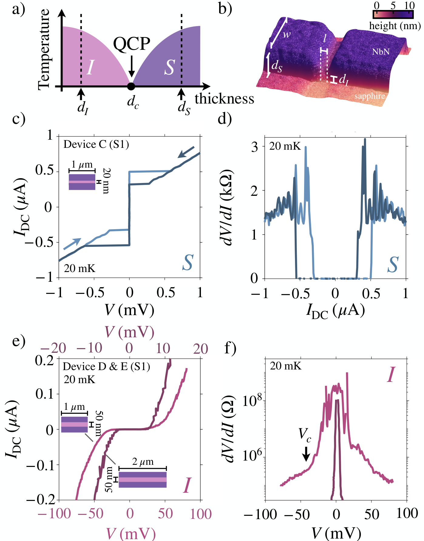
▲ (a) Thickness-controlled SIT phase diagram, with the boundary between the superconducting and insulating regions near \(d_{c}\). (b) An atomic force microscopy (AFM) image of the weak link, showing the thinned central region and the thicker electrodes on either side. (c, d) Short weak links with a length of \(20\,\mathrm{nm}\) carry a tunneling supercurrent. (e, f) When the thinned region is extended to \(50\,\mathrm{nm}\), superconducting tunneling is no longer observed, and resistive behavior appears.
Ref: C. G. L. Bøttcher et al., arXiv:2510.19983v1, Fig. 2. Original figure.

Two Fabrication Sequences for Weak Links

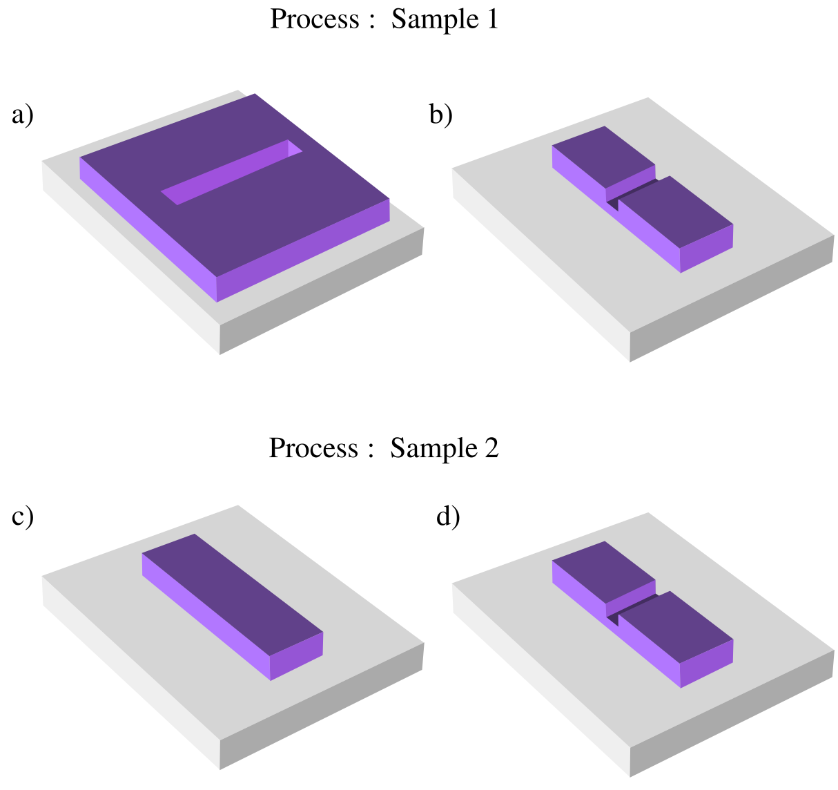
▲ (a→b) For Sample 1, a long trench is first etched into the NbN film to locally reduce its thickness, and the surrounding material is then removed. (c→d) For Sample 2, the wire is patterned first, and a short section in the middle is then locally thinned. Both processes form a weak link, but the wire sidewalls are exposed differently during subsequent processing. The two sets of samples show different distributions of supercurrent.
Ref: C. G. L. Bøttcher et al., arXiv:2510.19983v1, Fig. S8. Original figure.

Spectroscopy of the Planaron Qubit

Connecting the NbN weak link to a capacitor forms a Planaron. The junction is about \(1\,\mu\mathrm{m}\) wide and \(30\,\mathrm{nm}\) long; panel (a) below shows the circuit layout. When microwaves on the transmission line are resonant with the qubit, the amplitude and phase of the transmitted signal change. The qubit frequency can therefore be determined from the transmission coefficient \(S_{21}\).

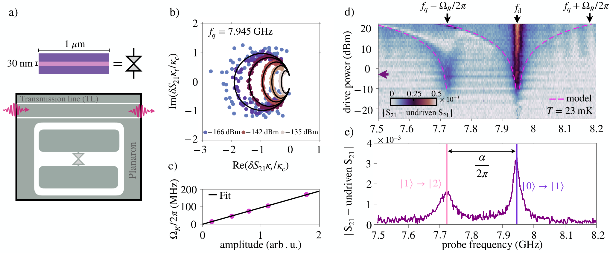
▲ (a) The weak-link geometry is shown above, with the capacitor and transmission-line layout below. (b) Complex transmission responses at different drive powers. As the power increases, the two-level transition gradually saturates, compressing the curves. (c) Fitting the transmission response in (b) to a two-level model gives the Rabi frequency \(\Omega_R\), which increases with the microwave drive amplitude. (d) With the \(|0\rangle \rightarrow |1\rangle\) transition continuously driven, a second microwave tone is swept to reveal the \(|1\rangle \rightarrow |2\rangle\) transition. Energy-level splitting also appears under strong driving. (e) A line cut at fixed power shows two peaks separated by about \(235\,\mathrm{MHz}\), giving the magnitude of the anharmonicity.
Ref: C. G. L. Bøttcher et al., arXiv:2510.19983v1, Fig. 3. Original figure.

\(T_1\) of the Planaron Qubit

In a later talk, Bøttcher presented measurements of the Planaron's energy relaxation time \(T_1\). The qubit is first excited to \(|1\rangle\) and then read out after different waiting times. The decay of the excited-state population gives \(T_1\). The result shown on the slide is \(T_1=243\pm7.9\,\mu\mathrm{s}\).[2]

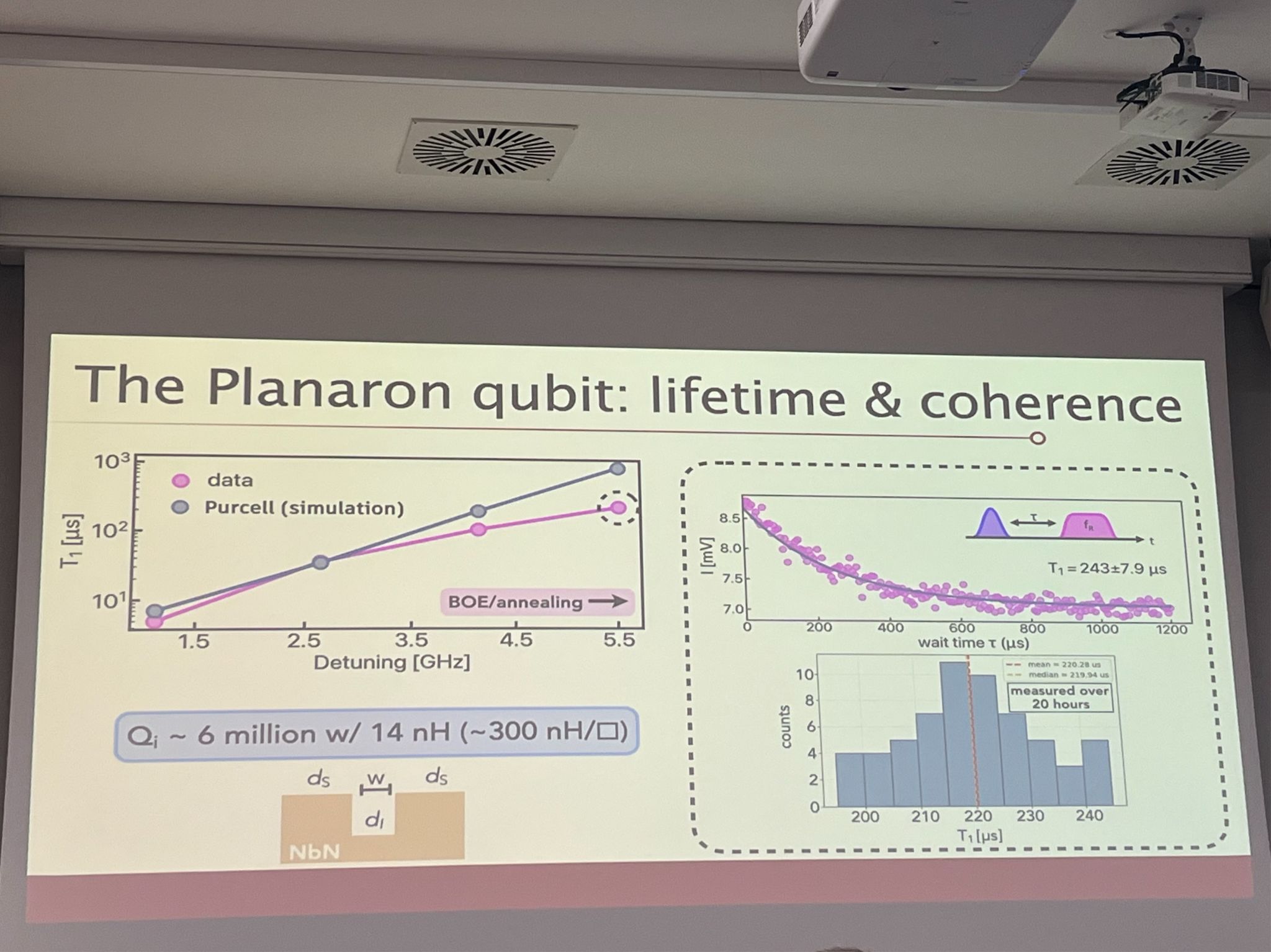
▲ The left plot compares \(T_1\) at different detunings. Pink points are experimental data, and gray-blue points are simulations of the Purcell effect. The upper-right plot shows the decay of the readout signal with waiting time. The lower-right plot shows the distribution of repeated \(T_1\) measurements over 20 hours, with a mean of about \(220\,\mu\mathrm{s}\). The slide does not specify the measurement temperature.
Ref: Charlotte Bøttcher, “The Planaron qubit: lifetime & coherence,” presentation slide; photo source: Michaela Eichinger, original LinkedIn post.

References

1. C. G. L. Bøttcher et al., “A transmon qubit realized by exploiting the superconductor-insulator transition,” preprint (2025). arXiv:2510.19983v1.
2. Charlotte Bøttcher, “The Planaron qubit: lifetime & coherence,” photograph of a presentation slide shared by Michaela Eichinger in the original LinkedIn post.

Originally written in Chinese by the author, these articles are translated into English to invite cross-language resonance.