Introduction to Superconducting Quantum Computers
Regarding superconducting quantum computers and superconducting qubits, 𝒊𝑁𝑆𝐼𝐺𝐻𝑇 𝒊ℏ has dedicated articles in the following series:
Interested readers can explore those sections. Here, we will use an overview to go through the concepts relevant to this workshop.
Josephson Junction
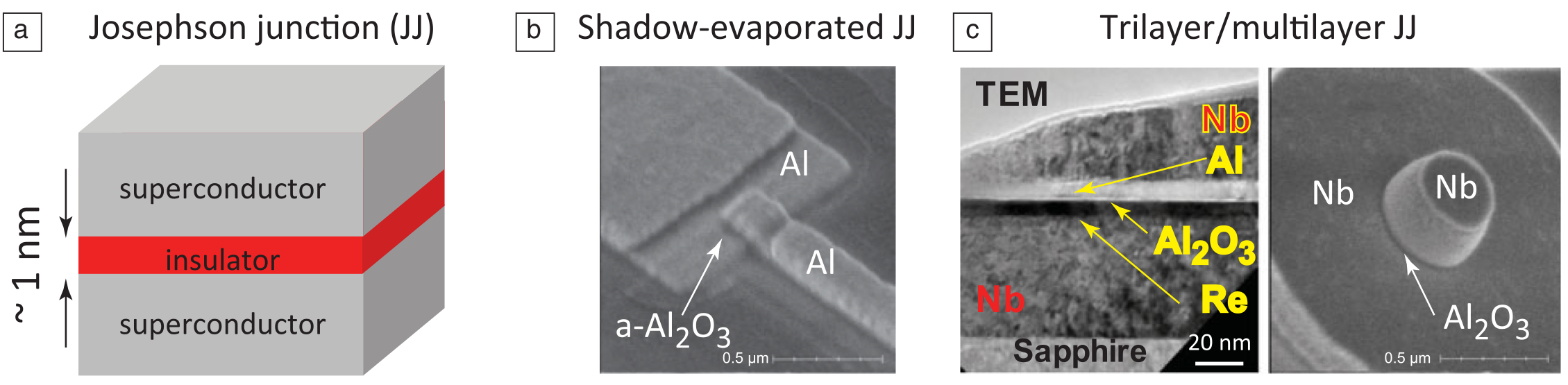
▲ Qubits made from superconductors are essentially inseparable from the Josephson Junction. A Josephson Junction is a sandwich-like structure featuring a non-superconducting material placed between two superconductors. Due to quantum effects, a superconducting current can pass through this non-superconducting layer via the tunneling effect. Common fabrication materials are aluminum-based (Al) or niobium-based (Nb). After depositing a layer of superconducting metal on a substrate, the surface is allowed to oxidize to form a thin oxide layer (i.e., the insulating non-superconducting layer), and then another layer of superconducting metal is deposited. This forms a Josephson Junction. This superconductor-insulator-superconductor structure is known as an SIS junction (Superconductor-Insulator-Superconductor).
Ref: 10.1557/mrs.2013.229
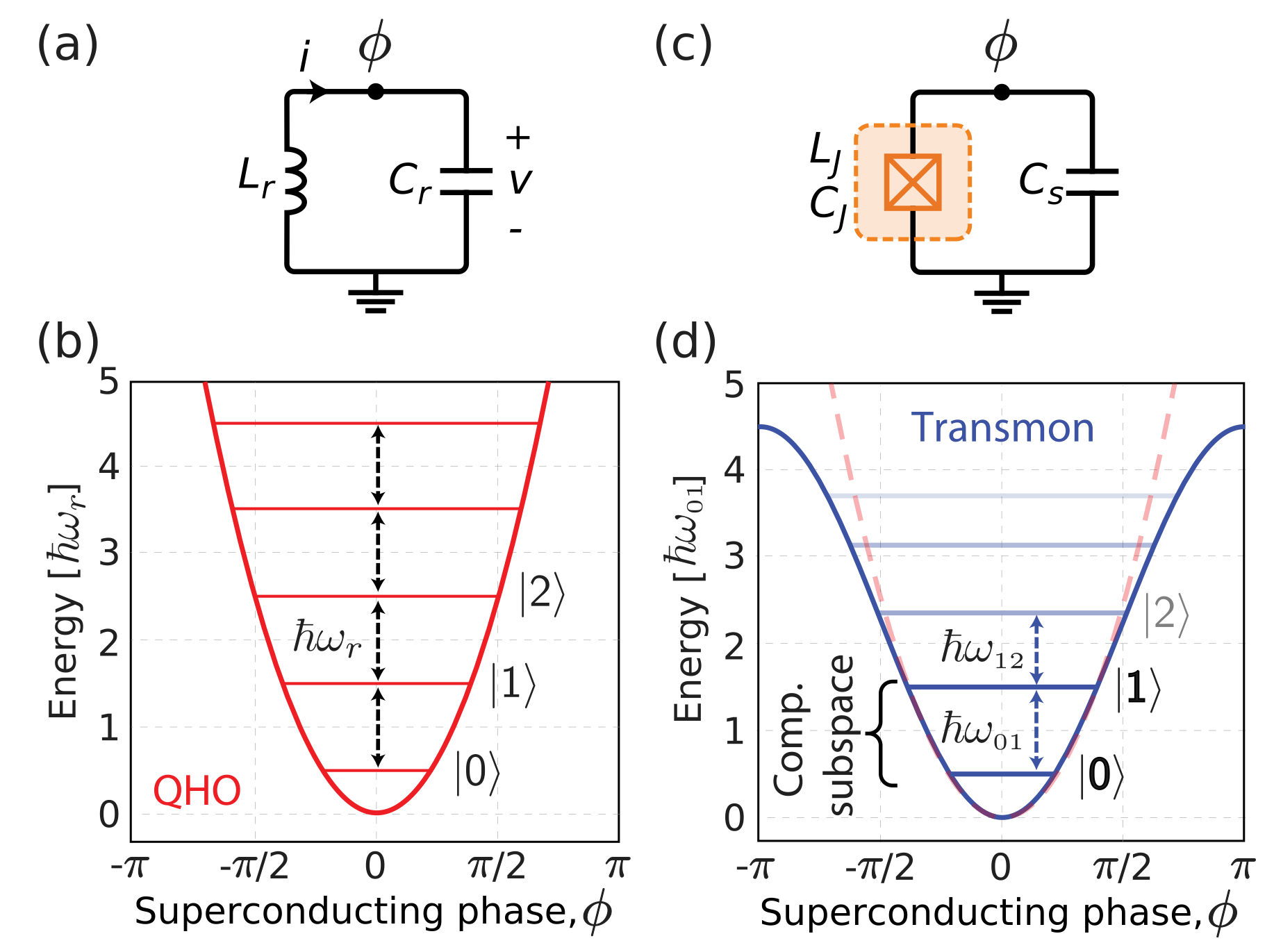
Superconducting Qubits
In classical computing, a series of classical bits uses two states, 0 or 1, to record information. Similarly, qubits also use different quantum states to record information and perform calculations. The simplest concept of quantum energy levels is the Quantum Simple Harmonic Oscillator. Since energy level simple harmonic oscillations are discrete in the quantum world, different energy levels can be used to represent information. By utilizing a Josephson Junction as a nonlinear inductive component to create quantum energy levels, we can isolate \( \ket{0} \) and \(\ket{1}\) using the distinct characteristics of these energy levels, where \(\hbar \omega_{01}\) is the eigenfrequency of the qubit. The most basic superconducting qubit simply consists of a superconducting capacitor and a Josephson Junction!
Ref: 10.1063/1.5089550
Controlling Qubits
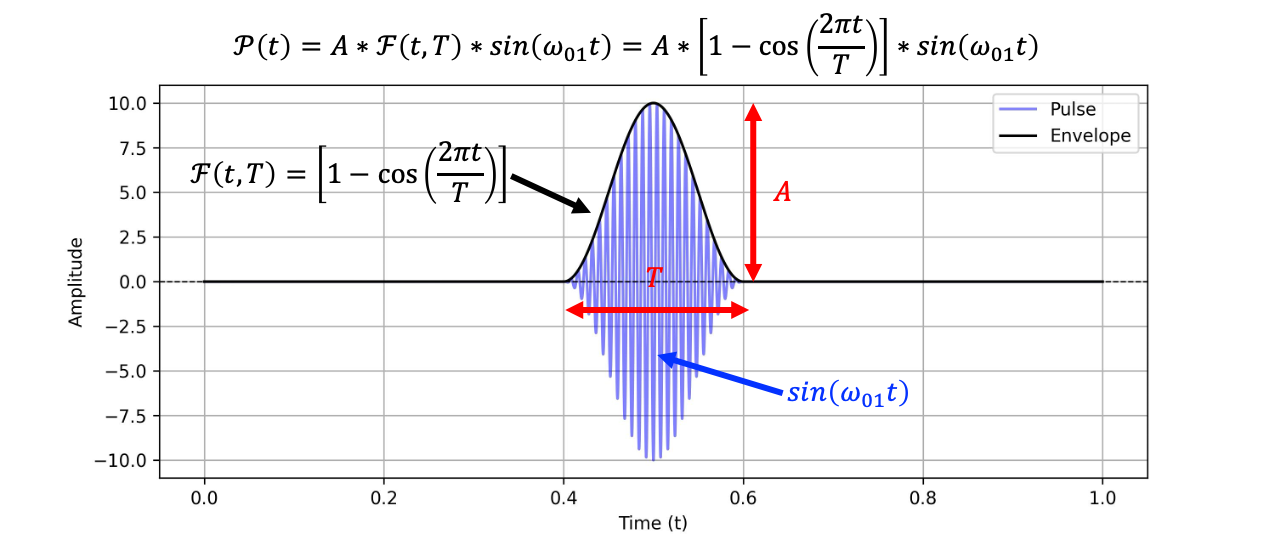
Main Parameters for Controlling a Qubit
- Pulse Amplitude (Amplitude \( A \)): Changes the state of the Qubit (rotation angle on the Bloch sphere).
- Pulse Duration (Duration \( T \)): Changes the state of the Qubit (rotation angle on the Bloch sphere).
- Pulse Frequency (Frequency \( \omega_d \)): Determines whether the Qubit can be driven accurately; the closer to the qubit's eigenfrequency \(\hbar \omega_{01}\), the better.
- Pulse Envelope (Envelope \( F(t, \tau) \)): Affects leakage.
A complete pulse can be expressed as: \[ P(t) = A \cdot F(t, \tau) \cdot \sin(\omega_{01} t) \] Examples are as follows:
This can be visualized using the Bloch sphere. Here, we illustrate rotations around the \( X \)-axis for \(0.25\pi\), \( 0.5\pi \), \(0.75\pi\), and \(\pi\)-pulses. As you can see, the magnitude of the amplitude determines the rotation angle.
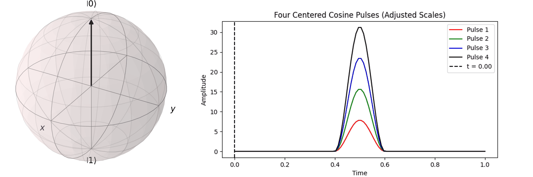
Similarly, we can also discuss using different pulse durations \(T\) to achieve the same \( \pi \)-pulse from \( |\ 0\rangle \rightarrow |\ 1\rangle \).
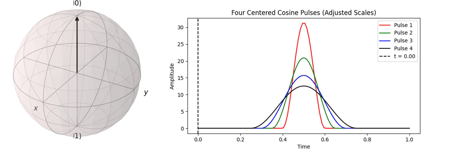
Generally, because the coherence time of a Qubit is very short, we want to complete the Qubit operations in the shortest possible time. For superconducting qubits, maintaining a coherence time in the microseconds (μs) range is already considered quite long with current technology. Therefore, superconducting qubit pulses are mostly fixed at the nanosecond (\(ns\)) scale. Thus, manipulating the state of a Qubit generally relies on adjusting the pulse amplitude to determine the rotation angle.
(In experiments, driving takes about \(10ns\)a)
\(^a\) 10.1103/PRXQuantum.5.030353
In practice, determining the pulse duration \(T\) and amplitude \(A\) is a routine part of daily Qubit calibration. Proper calibration yields high-quality quantum computing results; conversely, errors alone can cause calculations to be less accurate than classical computers.
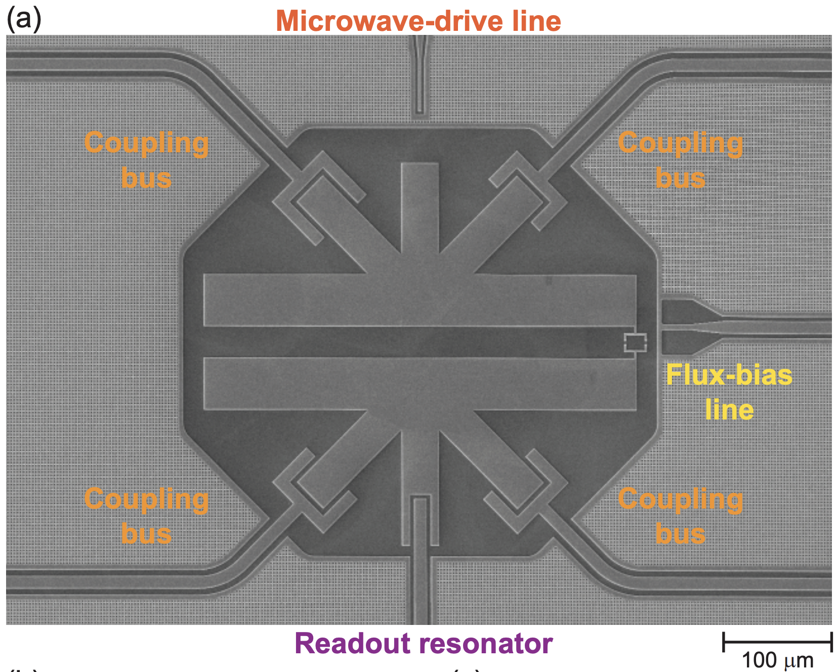
Single Qubit Drive and Readout Circuit
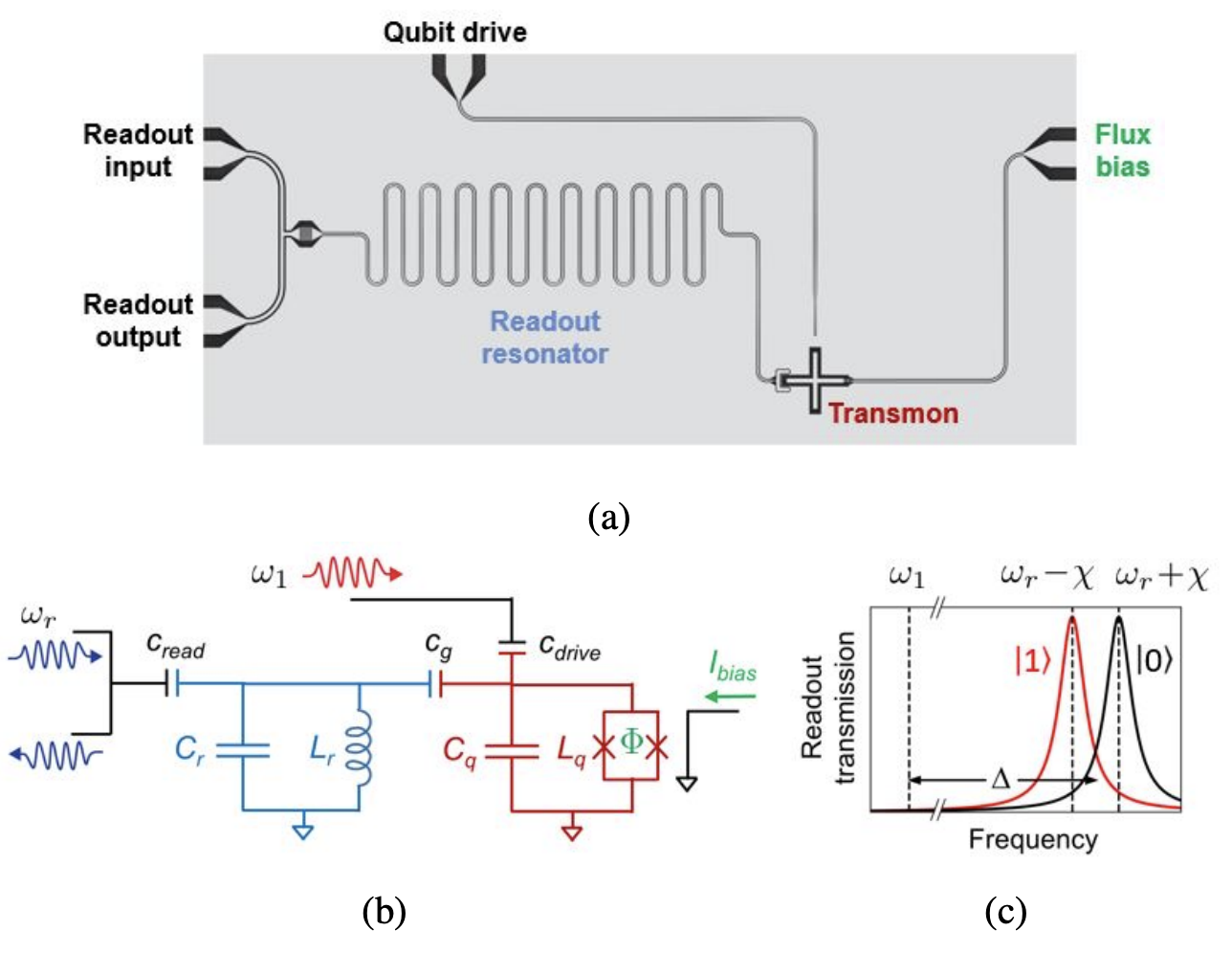
▲ Transmon circuit layout. (a) Circuit diagram under a microscope, (b) Corresponding circuit diagram. In this diagram, there is one Qubit (red Transmon) and one readout resonator (sky blue). Two feedlines individually drive the qubit and the readout resonator. The components are coupled using capacitors. Additionally, a Flux line is connected next to the Qubit, which generates a magnetic field to alter the Transmon's operating frequency. (c) Because the readout resonator is coupled to the qubit, it experiences a spectral shift depending on whether the qubit is in the \(|0\rangle\) or \(|1\rangle\) state. We use this characteristic spectral shift of the readout resonator to determine the state of the qubit.
arxiv.org/pdf/2106.11352
Couplers
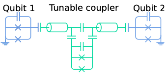
The Resonator/Coupler facilitating interactions between qubits can be tunable, allowing for further adjustment of the coupling strength between different Qubits, though this also increases the complexity of the control circuit.
arxiv: 2408.12433
Superconducting Quantum Chips
A complete superconducting quantum computer requires at least: a Helium-3 ultra-low temperature vacuum environment, a cooling system, and a massive array of RF signal control and readout instruments, making current superconducting quantum computers extremely large. Furthermore, a single qubit requires at least four lines:
- Control Frequency * 1: A Flux line to adjust magnetic flux.
- Control State * 1: A Drive line.
- Readout State * 2: Readout lines (one in, one out).
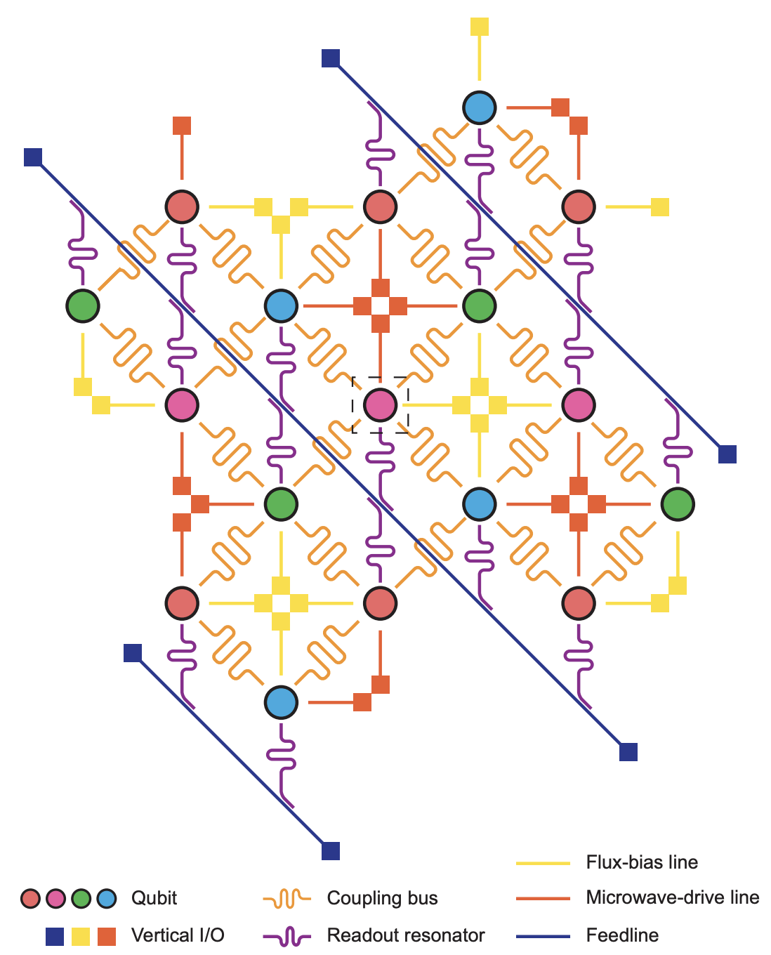
▲ To achieve quantum computing, many Qubits must be operated simultaneously, and extra Qubits are required for error correction. The image above shows a 17-qubit experimental quantum chip arranged in a quantum error-correction format called a surface code. The circles represent Qubits: pink and red are Data Qubits, while sky blue and green are Check Qubits. Each Qubit is connected to 7 lines (nicknamed Starmon), which include 4 for inter-qubit coupling, 1 Flux line, 1 Drive line, and 1 Readout resonator. The Readout resonators are merged into three feedlines. Although current technology can multiplex the Readout lines of multiple Qubits together—sharing the same Readout line (the so-called Feedline) via frequency isolation techniques—we still need to account for the Resonators that control interactions between qubits. A 100-qubit quantum computer prototype requires 400 external lines, which is why a massive tangle of wiring is a common sight in current superconducting quantum computers.
https://arxiv.org/pdf/1612.08208
Superconducting Quantum Computer Architecture
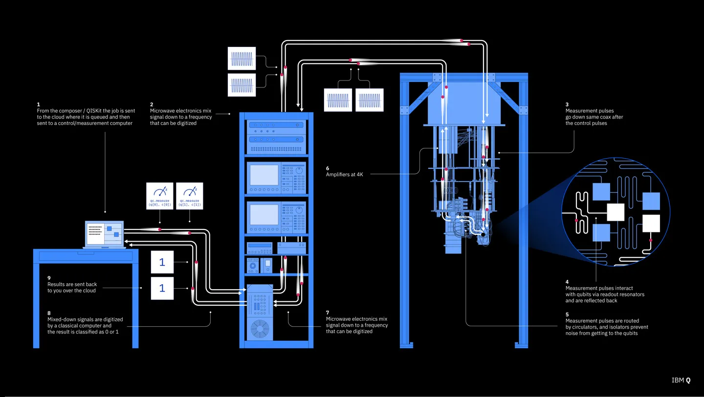
▲As superconducting quantum computers are still under development, they require operation at near-absolute-zero temperatures. A prototype machine is extremely large and expensive, and requires numerous electronic controllers to precisely manage individual qubits. Prototype machines from companies like IBM, Google, and IQM are accessible via the cloud, enabling external developers to explore new quantum applications. The diagram illustrates a quantum computing scenario using IBM's cloud-based quantum platform:
(1) Users submit commands via a cloud interface to IBM's system.
(2) These commands are translated by classical computers into control signals (via DAC: Digital-to-Analog Conversion) and sent through microwave electronics.
(3) Microwave pulses are transmitted into the cryogenic environment through superconducting coaxial cables.
(4) After processing by the quantum chip, output signals are sent back through readout loops.
(5) The readout loops include isolators to prevent signals from reflecting back into the qubits.
(6) The signals are amplified by quantum amplifiers.
(7) Signals are digitized and analyzed by room-temperature electronics (ADC: Analog-to-Digital Conversion).
(8) The instrument processes the data.
(9) Results are returned to the user.
Ref: IBM
Originally written in Chinese by the author, these articles are translated into English to invite cross-language resonance.
 Peir-Ru Wang