𝒊𝑁𝑆𝐼𝐺𝐻𝑇 𝒊ℏ
  • Home
  • Qubit Physics
    • Superconducting Qubits (Elementary)
    • Superconducting Qubits (Advanced)
    • Semiconductor Spin Qubits
  • Hardware
  • Quantum Industries
  • Workshop Note
    • 2026 Academia Sinica SCQC Winter Workshop
  • Consultance
    • Taiwan Market Outreach Services
    • About Us
  • 中文版

Computation Is Physical

  1. Home
  2. PHYS598500
← Previous Next →
QH-2026F v5 · 16-Week Overview
Week 1 Manual Slides · Computation Is Physical | QH-2026F v5
Week 2 Manual Slides v41 · Hardware, Superconductivity, and Josephson Anharmonicity | QH-2026F v5
𝒊𝑁𝑆𝐼𝐺𝐻𝑇 𝒊ℏ

Exploring the Quantum Technology Together.

𝐾𝐸𝐸𝑃 𝐼𝑁 𝑇𝑂𝑈𝐶𝐻

  • info@insight-ihbar.com

𝒊𝑁𝑆𝐼𝐺𝐻𝑇 𝒊ℏ

All Rights Reserved

PHYS598500 · Week 1 · T1

Computation Is Physical

T1 · How Computation Becomes Physical Operations

T1 roadmap: How Computation Becomes Physical Operations
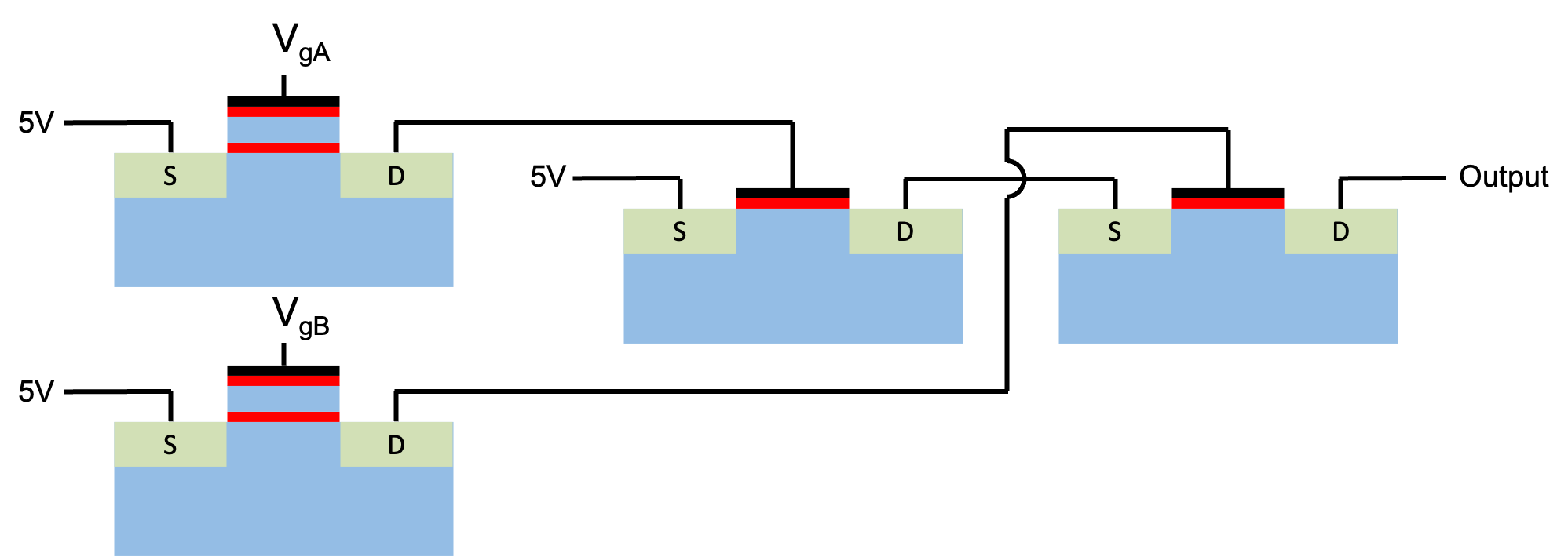
Floating-gate transistor network used to represent an AND calculation
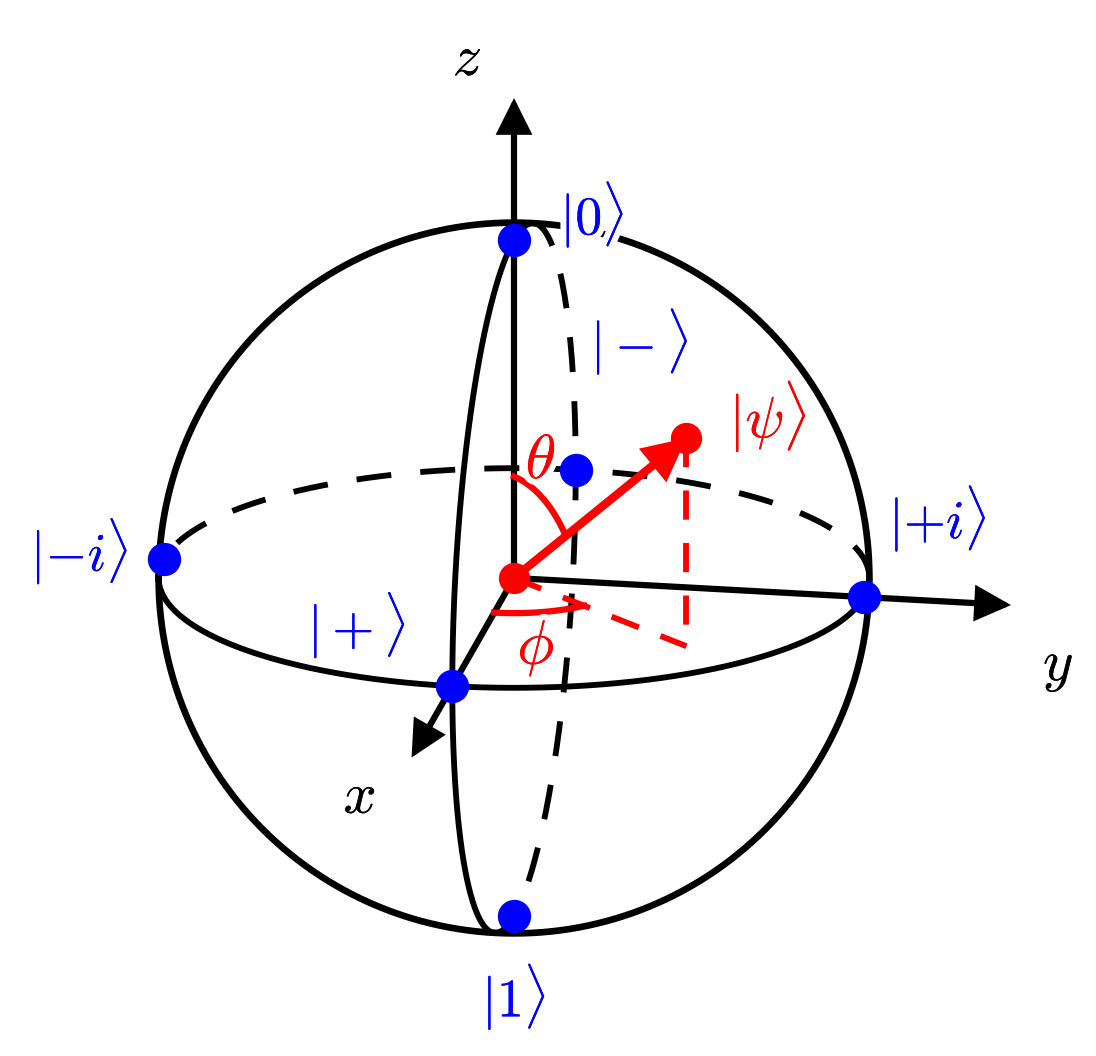
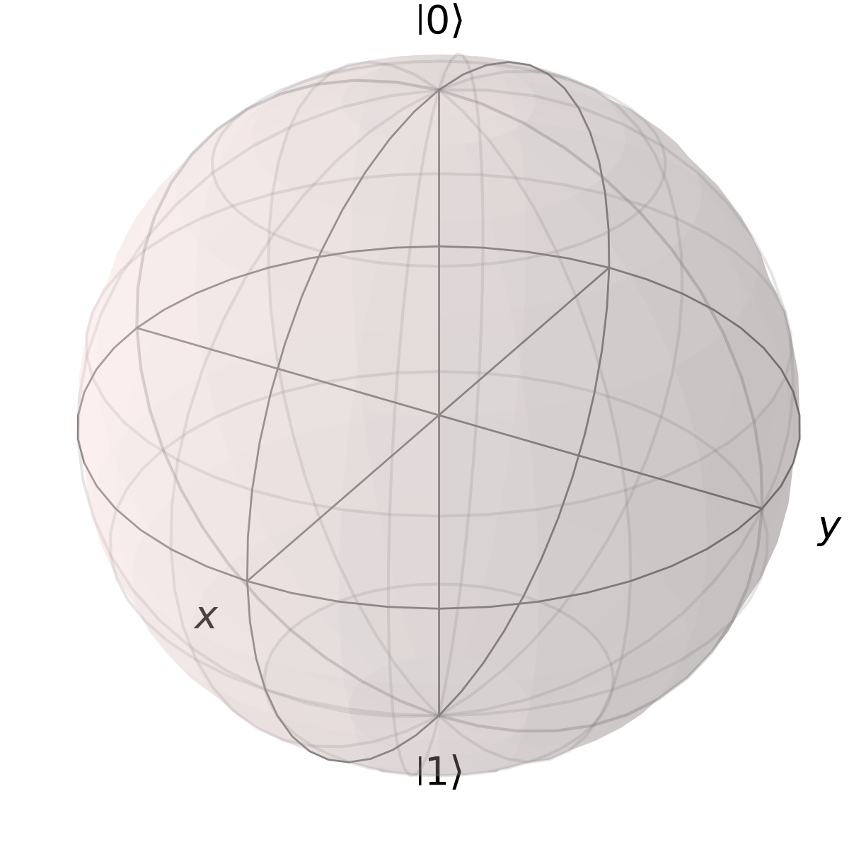
Bloch sphere with the six Pauli eigenstates and a general state labelled by theta and phi

T2 · Fabricating Qubits from Circuits
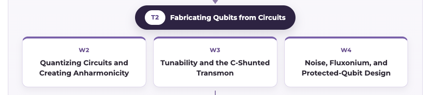
T2 roadmap: Fabricating Qubits from Circuits
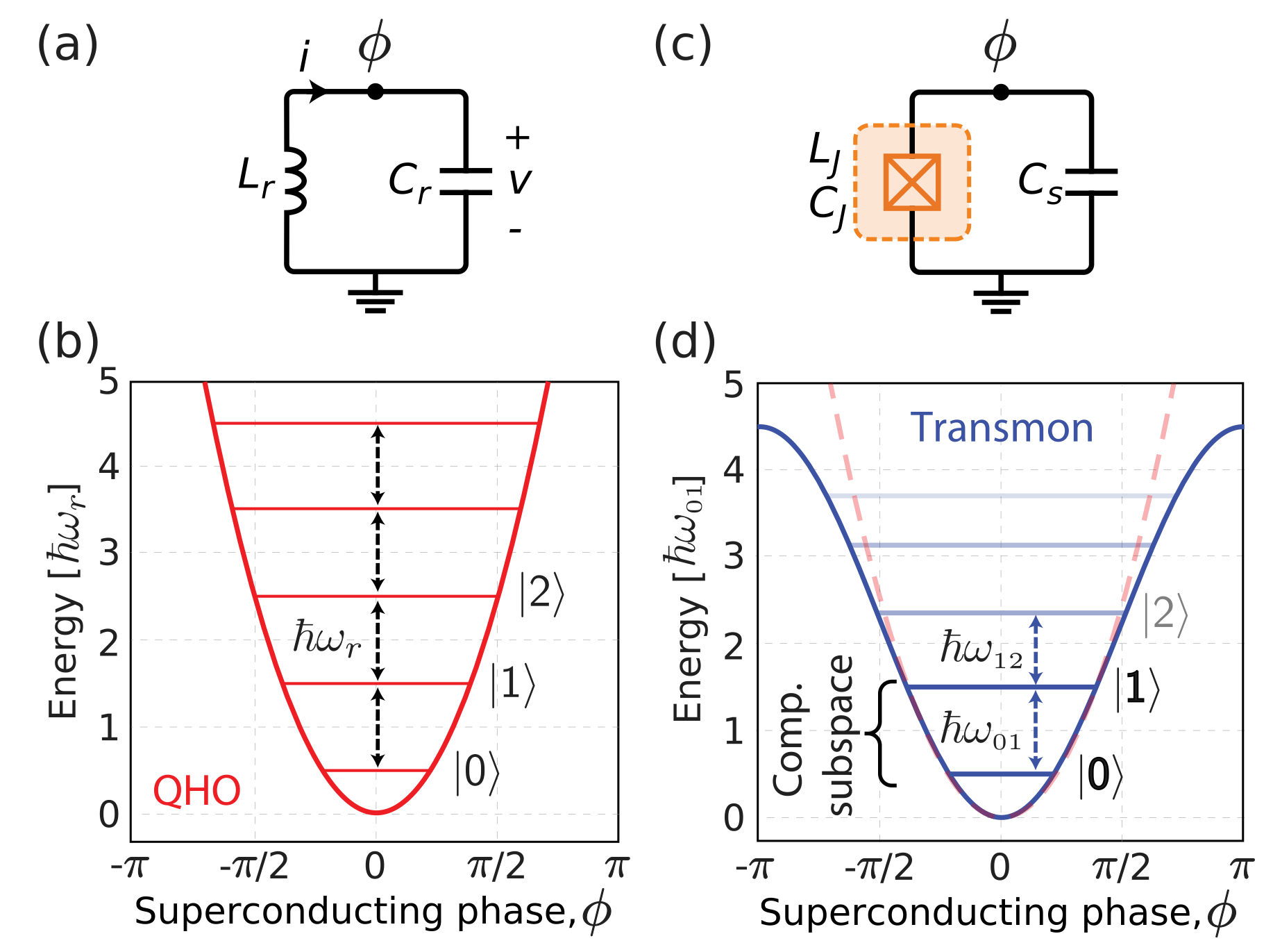
Superconducting-circuit energy levels and qubit-state diagrams

T3 · Controlling, Coupling, and Reading Out Qubits
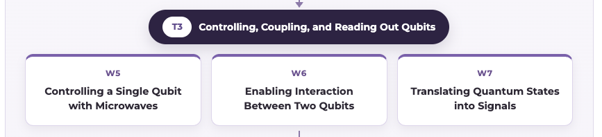
T3 roadmap: Controlling, Coupling, and Reading Out Qubits
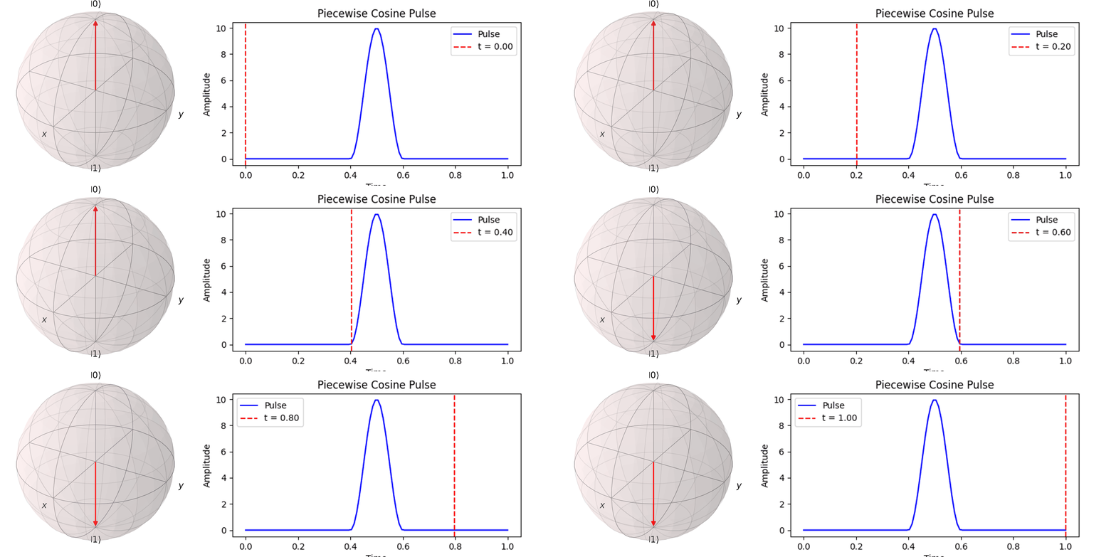
Animated microwave-pulse control of a qubit on the Bloch sphere

T4 · Calibration, Verification, and Quantum Error Correction
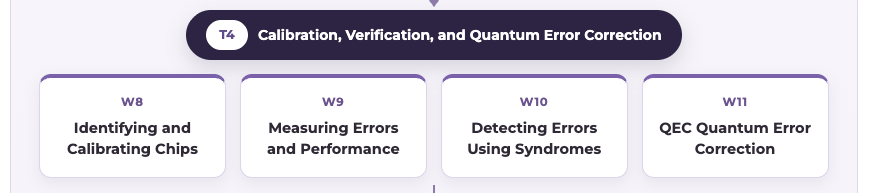
T4 roadmap: Calibration, Verification, and Quantum Error Correction
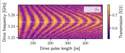
Chevron calibration plot of qubit transmission versus drive frequency and pulse length

T5 · Stabilizing Designs into Chips
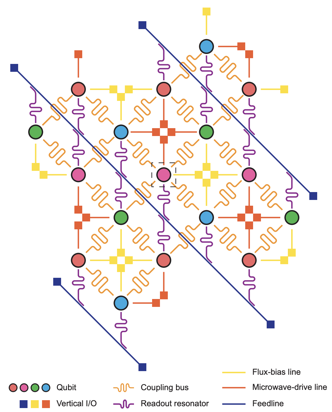
T5 roadmap: Stabilizing Designs into Chips
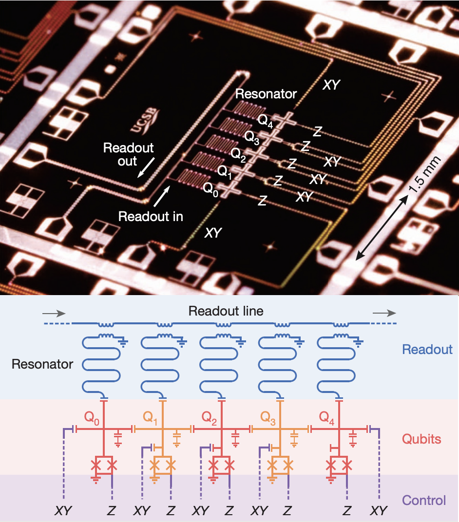
Superconducting-qubit chip surface and fabrication layout Five-qubit superconducting processor layout

T6 · Cryogenics, Signal, and System Integration

T6 roadmap: Cryogenics, Signal, and System Integration
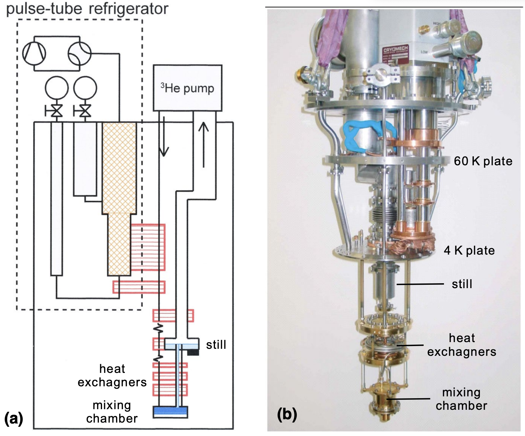
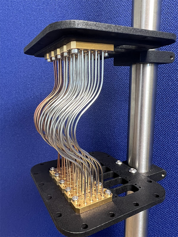
Cryogenic quantum-computing signal-chain integration Cryogenic coaxial wiring installed in a dilution refrigerator

T7 · Integrating a Complete Quantum Computer

T7 roadmap: Integrating a Complete Quantum Computer
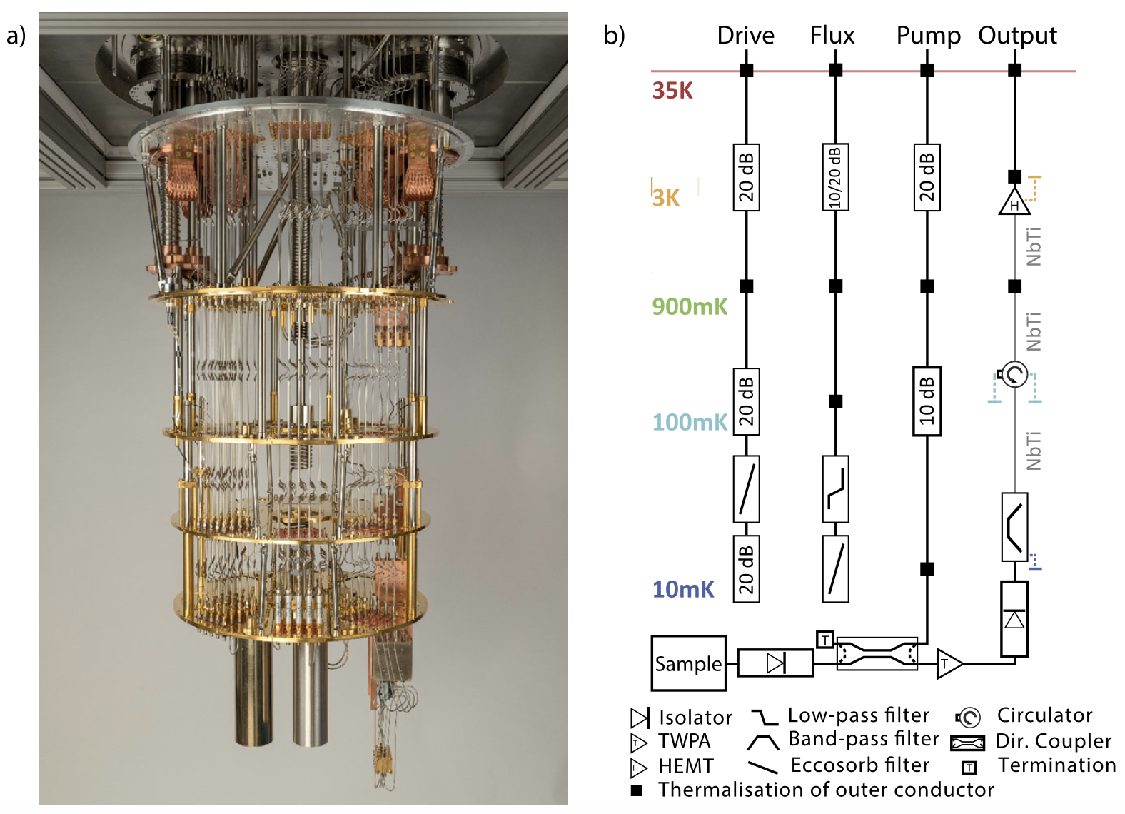
Integrated architecture of a complete superconducting quantum computer

Let's start!

Why Must Computer Science Eventually Meet Physics?

→Because computation needs hardware.

In physics, we study:

Matters ← the hardware itself
Energy transfer ← how we control the hardware
State evolution ← how the algorithm is encoded

Can Calculation and Reasoning Be Mechanized?

From Human Procedure to Programmable Machine

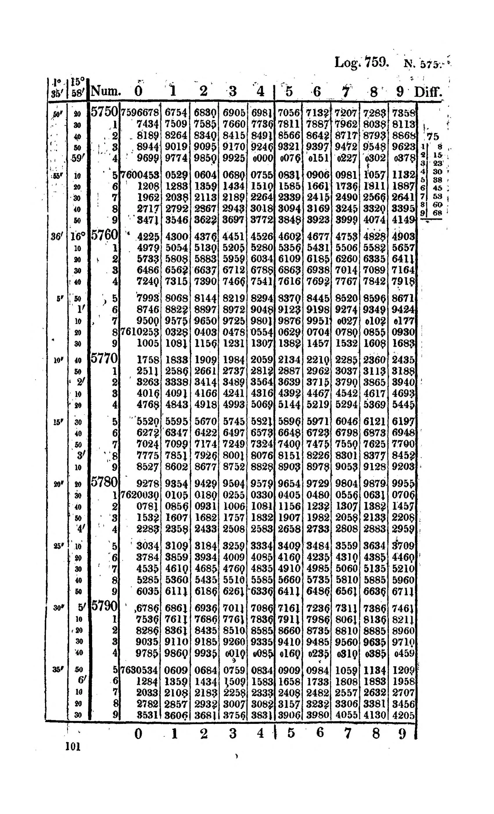
Lookup Tables have Errors
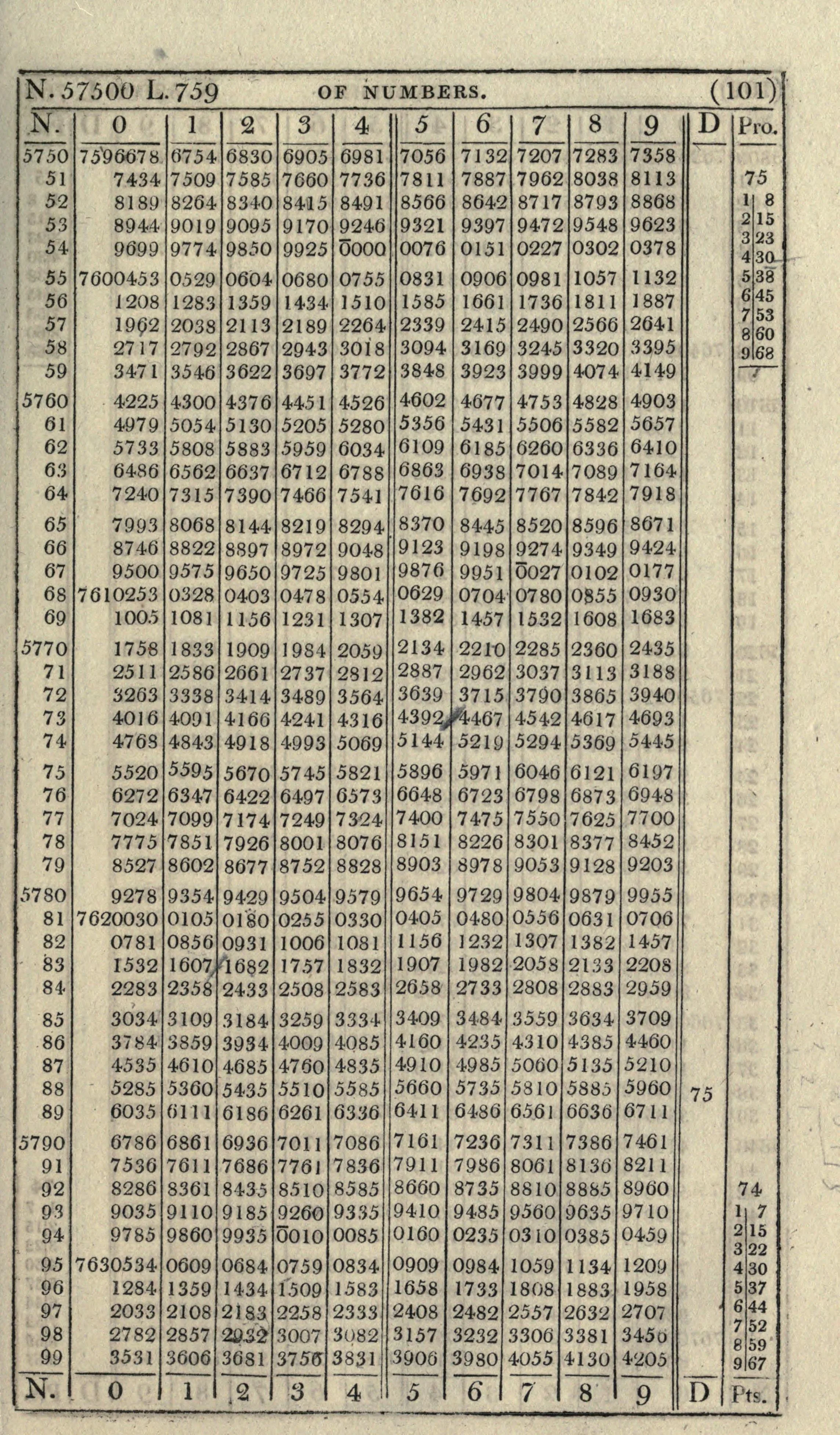
Hutton 1811 · page 101 · two wrong last digits
Charles Hutton's 1811 logarithm table, page 101
Hutton table row containing the wrong last digits for 57628 and 57629 wrong
Babbage 1827 · page 101 · corrected values
Charles Babbage's 1827 logarithm table, page 101
Babbage table row containing the corrected last digits for 57628 and 57629 correct

Seven-place common (base-10) logarithms: the page prints only the last four mantissa digits, the leading \(760\) coming from the block header N. 57500 L. 759.

\(\log_{10}57628=4.7606335\)Hutton …6336 \(\log_{10}57629=4.7606411\)Hutton …6410

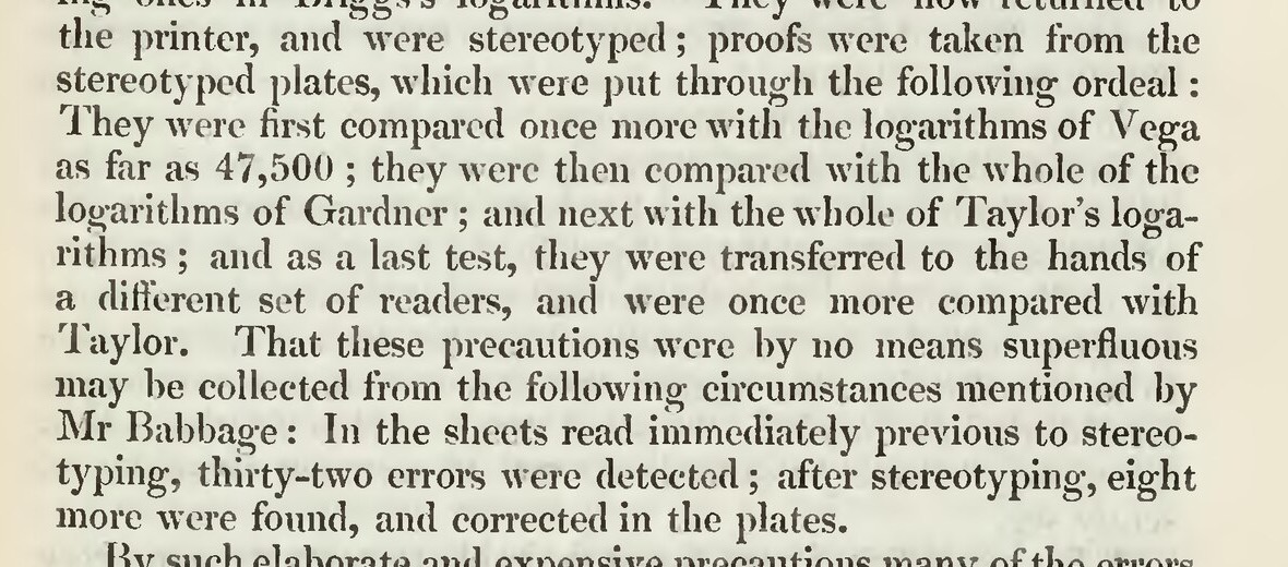
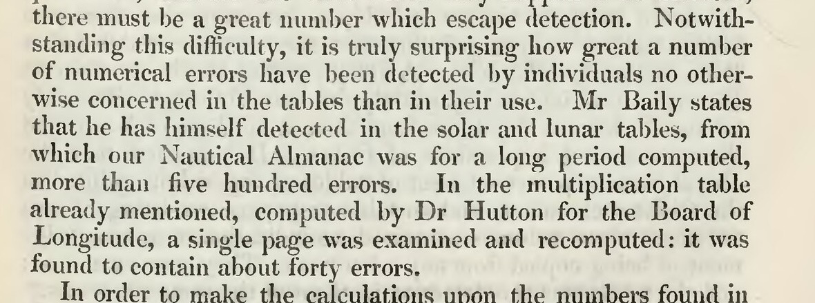
Why Mechanize Tables? Too many errors
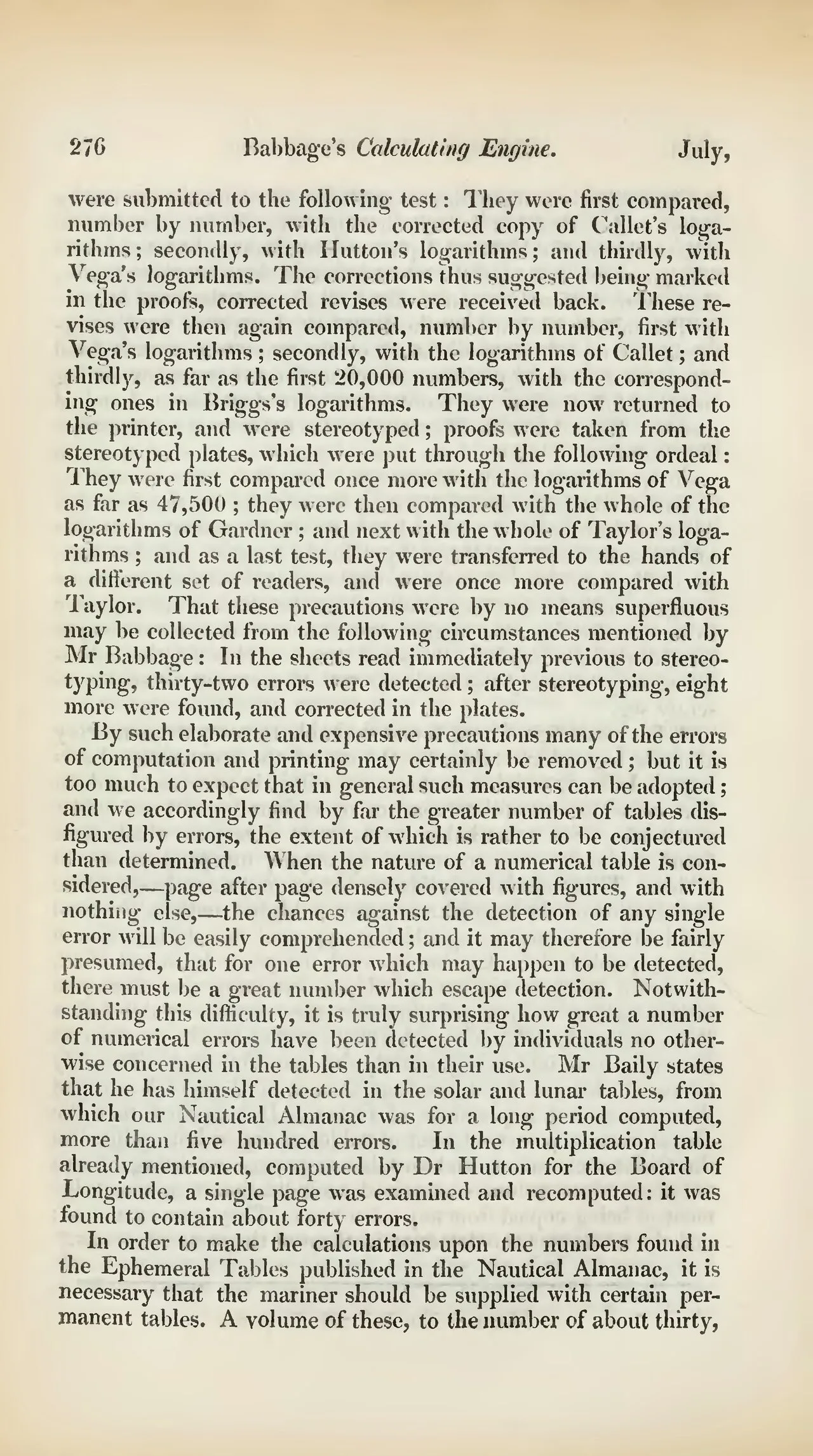
The Edinburgh Review, July 1834, page 276
Enlarged passage reporting errors found before and after stereotyping
32 + 8 errors

Thirty-two errors were caught just before stereotyping; eight more remained after the plates were made.

Enlarged passage reporting more than 500 errors and about 40 errors on one table page
>500 errors

More than 500 errors were found in solar and lunar tables.

The Edinburgh Review, vol. 59 · July 1834

Charles Babbage: From Automatic Tables to a Programmable Machine

Charles Babbage (1791–1871) first designed the Difference Engine to automate numerical tables. Finite differences reduce polynomial tabulation to repeated addition, making the task suitable for a gear-based mechanism and reducing human calculation and typesetting errors.

The later Analytical Engine was a general architecture. It separated a “store” from a “mill,” used punched cards to specify operations and data, and included sequencing, repetition, and conditional control.

The full Analytical Engine was not completed in Babbage's lifetime.
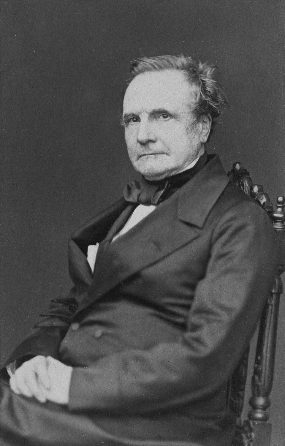
Portrait of Charles Babbage, circa 1860

Ref: https://en.wikipedia.org/wiki/Charles_Babbage

▲
Ref: https://en.wikipedia.org/wiki/Charles_Babbage


Difference Engine No. 2: From Drawings to Mechanism
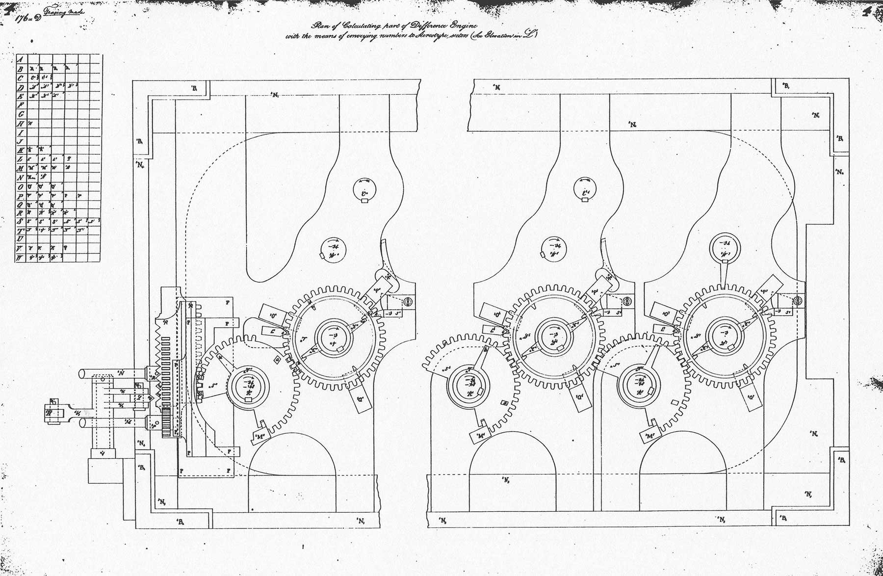
Plan of the calculating part of Babbage's Difference Engine

Plan of the calculating mechanism
Ref: Cronatec · How did the Difference Engine work?

▲
Ref: https://cronatec.ch/how-did-the-difference-engine-work/
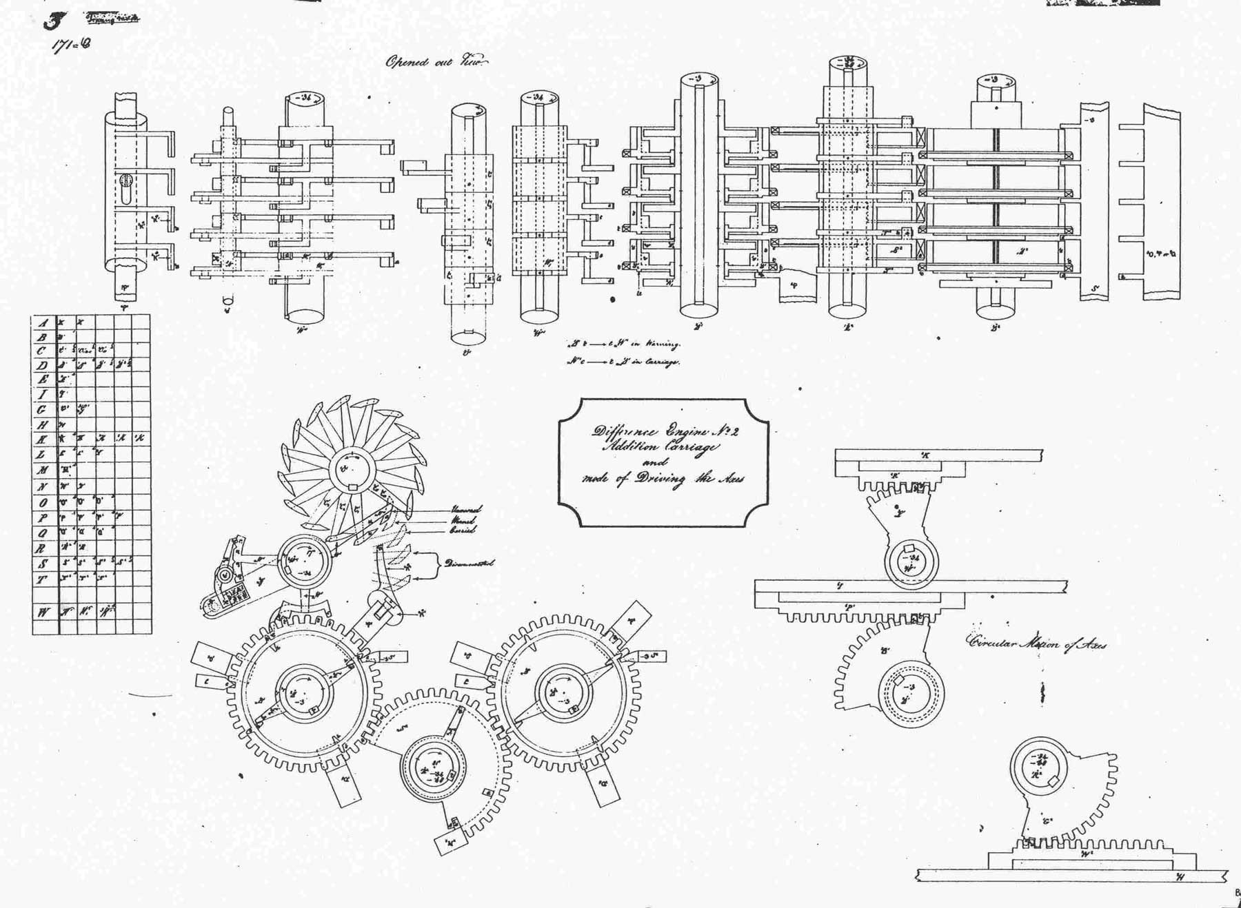

Mechanical drawings of the addition and carriage mechanisms in Difference Engine No. 2

Addition and carriage mechanisms
Ref: Cronatec · How did the Difference Engine work?

▲
Ref: https://cronatec.ch/how-did-the-difference-engine-work/


Difference Engine No. 2: Built in Metal
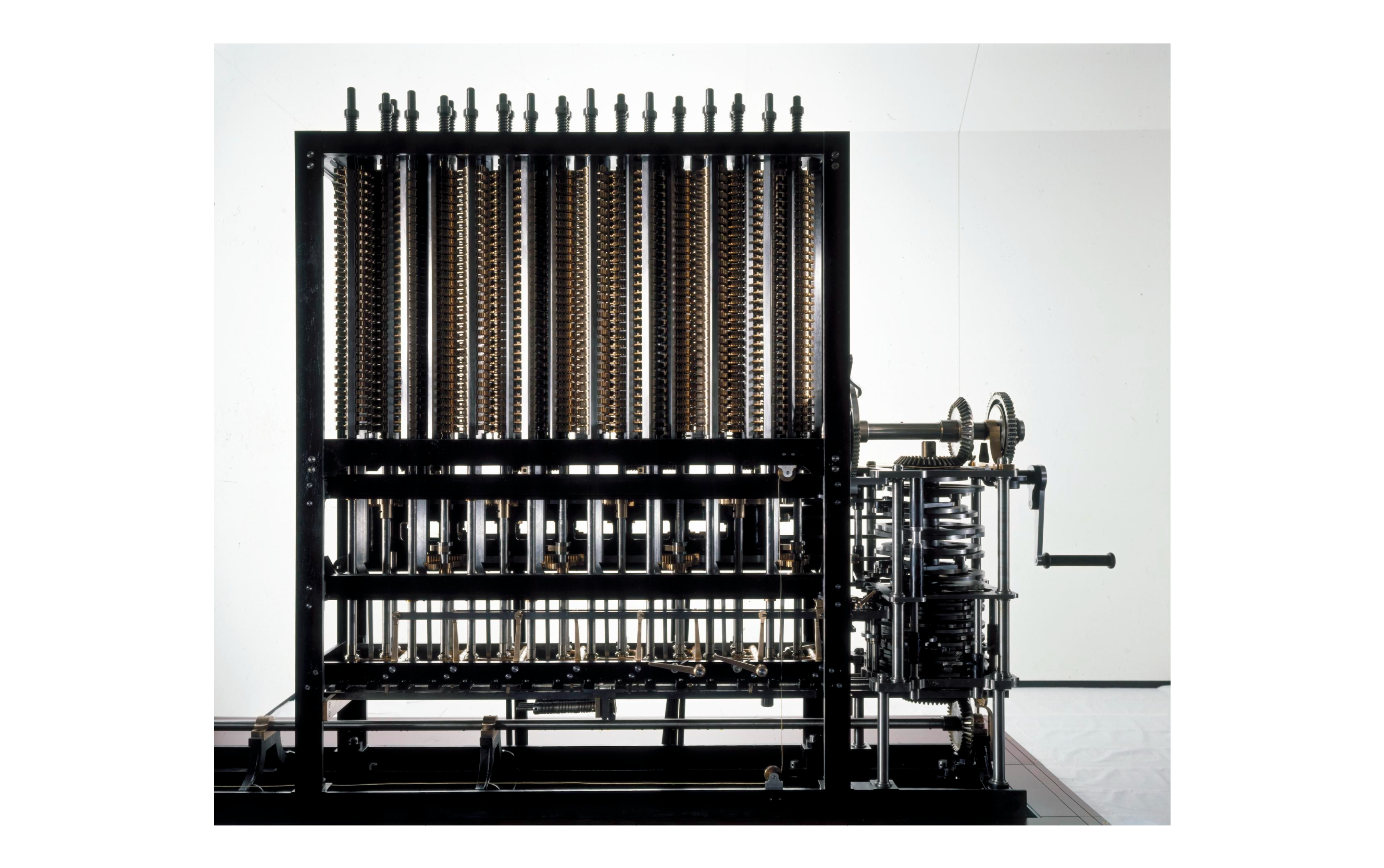
The complete Difference Engine No. 2 reconstructed by the Science Museum

Complete reconstruction
Ref: Science Museum Group Collection

▲
Ref: https://collection.sciencemuseumgroup.org.uk/objects/co62748/babbages-difference-engine-no-2-2002


Close-up of decimal figure wheels and gear trains in Difference Engine No. 2

Decimal figure wheels and gear trains
Ref: Science Museum Group Collection

▲
Ref: https://collection.sciencemuseumgroup.org.uk/objects/co62748/babbages-difference-engine-no-2-2002


Analytical Engine: Mechanism and Punched-Card Control

Sketch elevation of the driving and directive mechanism of the Analytical Engine, 1841
Driving and directive mechanism, 1841
Ref: Science Museum Group Collection
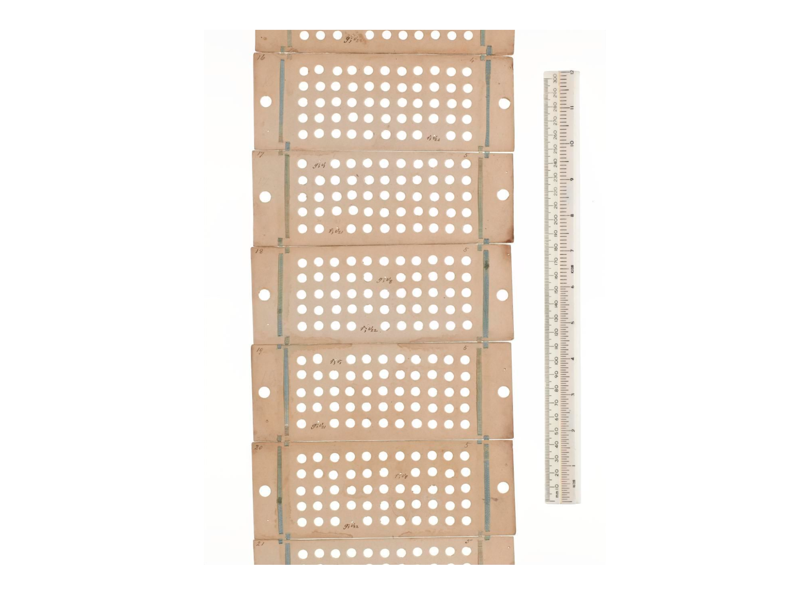
Punched cards used to encode operations and variables for Babbage's Analytical Engine
Operation and variable punched cards
Ref: Science Museum Group Collection

Boolean Algebra: Logic Becomes Algebra

Boole showed that logical statements can be represented by symbols and manipulated with algebraic rules.

For Boolean variables \(a,b\in \{F,T\} \text{ or }\{0,1\}\), logical AND behaves exactly like multiplication:

Logic: \(a\ \mathrm{AND}\ b\)

\(a\)\(b\)\(a\land b\)
FFF
FTF
TFF
TTT

Algebra: \(a*b\)

\(a\)\(b\)\(a*b\)
000
010
100
111

For \(a,b\in\{0,1\}\), \(a\land b=a*b\).
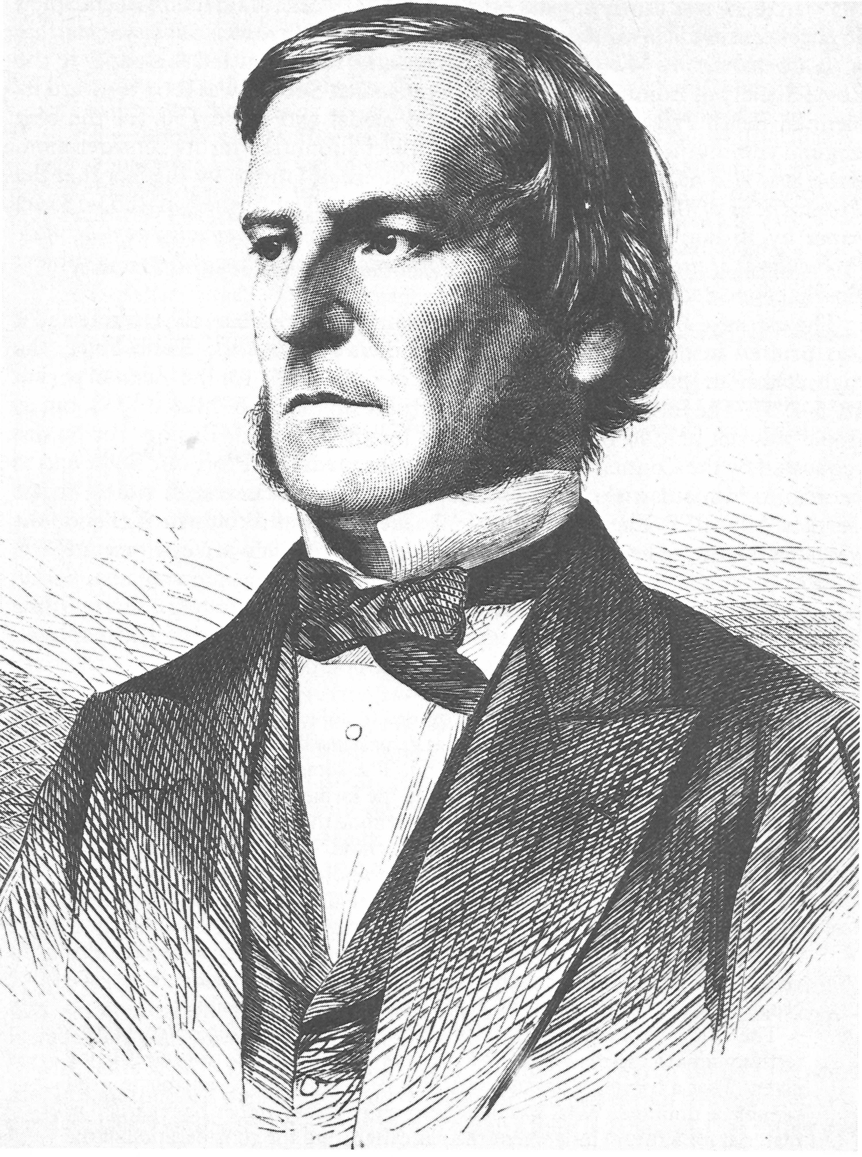
A B U
\(A\cap B\)
Portrait of George Boole

George Boole
Ref: Wikipedia

▲
Ref: https://en.wikipedia.org/wiki/George_Boole


Logic Gates Implement Boolean Functions

Let \(A=\{a=1\}\) and \(B=\{b=1\}\). The shaded region is where the output equals \(1\).
A U
\(A\)
A U
\(U\setminus A\)
A B U
\(A\cap B\)
A B U
\(U\setminus(A\cap B)\)
A B U
\(A\cup B\)
A B U
\(U\setminus(A\cup B)\)
A B U
\(A\mathbin{\triangle}B\)
A B U
\((A\cap B)\cup(A^c\cap B^c)\)
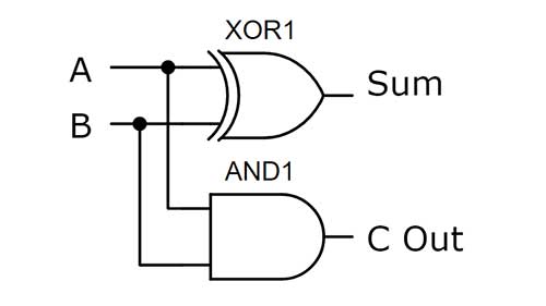
Half-adder circuit built from XOR and AND gates
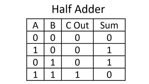
Half-adder truth table with Carry before Sum

Half adder: AND → Carry; XOR → Sum

Shannon: Boolean Algebra Becomes Switching-Circuit Design

Claude Shannon (1916–2001) showed that the ON/OFF behavior of relay circuits follows Boolean algebra. A switch is OFF when the circuit is open and ON when a conducting path is closed. We encode OFF as \(0\) and ON as \(1\).

Connection Boolean operation
Series: output is ON only when \(a\) and \(b\) are ON \(a\land b\)
Parallel: output is ON when \(a\) or \(b\) is ON \(a\lor b\)
Normally closed: output is ON when \(a\) is OFF \(\neg a\)

\[\boxed{\text{Boolean expression}\longleftrightarrow\text{switching network}.}\]

This made circuit design systematic: specify the desired ON/OFF output, express and simplify it with Boolean algebra, then connect switches that realize the same relation.

Portrait of Claude E. Shannon

Ref: https://en.wikipedia.org/wiki/Claude_Shannon

▲
Ref: https://en.wikipedia.org/wiki/Claude_Shannon


How we encode algorithm into physical evolution?

From Reversible Boolean Functions to Unitary and Hamiltonian Evolution

Semiconductor Fabrication
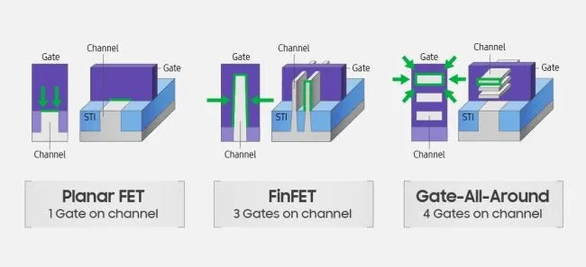
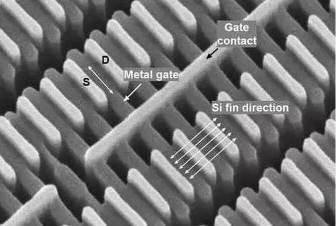
Planar FET, FinFET, and gate-all-around transistor structures
Electron micrograph of FinFETs with source, drain, metal gate, gate contact, and silicon fin labels
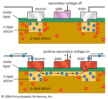
MOSFET with gate voltage off and no conducting channel between source and drain
MOSFET with positive gate voltage and a conducting channel between source and drain

Refs: Britannica · UTMEL · Deep Forest

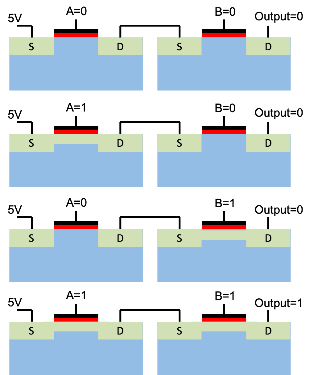
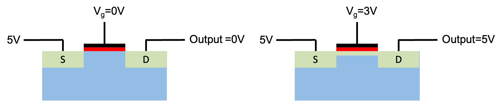
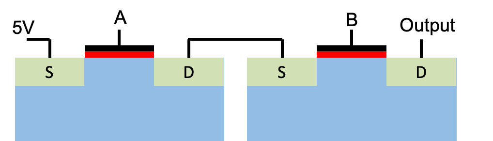
AND Gate:Series Switches
MOSFET with no positive gate voltage and no conducting channel
MOSFET with positive gate voltage and a conducting channel
Two transistor switches A and B connected in series between 5 volts and the output
AND gate symbol and truth table
Four AND-gate series-switch states: only A equals 1 and B equals 1 produces a 5 volt output

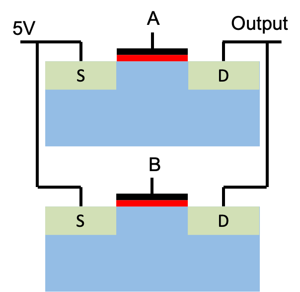
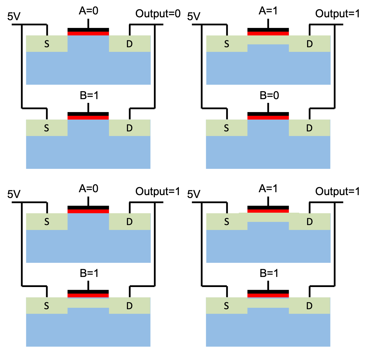
OR Gate:Parallel Switches

MOSFET with no positive gate voltage and no conducting channel
MOSFET with positive gate voltage and a conducting channel
Two transistor switches A and B connected in parallel between 5 volts and the output
OR gate symbol and truth table
Four OR-gate parallel-switch states: every case except A equals 0 and B equals 0 produces a 5 volt output

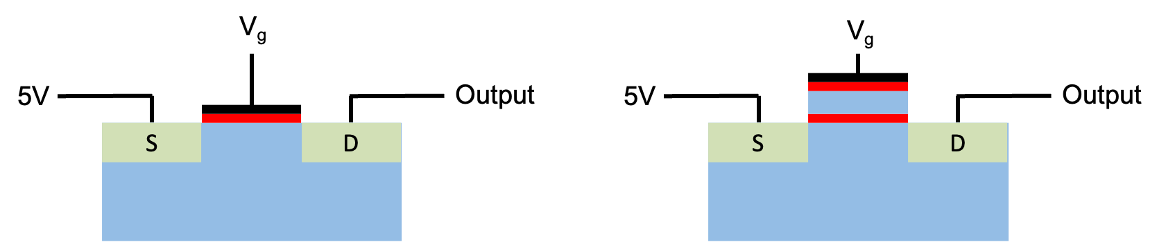
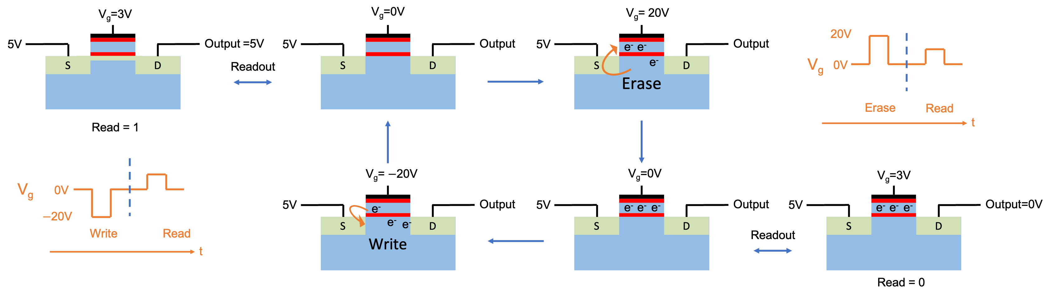
Flash Memory (I)

Memory adds one more floating gate.
Transistor and floating-gate memory transistor
Reading a floating-gate transistor

Flash Memory (II)

Memory adds one more floating gate.
Transistor and floating-gate memory transistor
Reading a floating-gate transistor
Flash-memory write, read, and erase cycle
Floating-gate transistor network used to represent an AND calculation
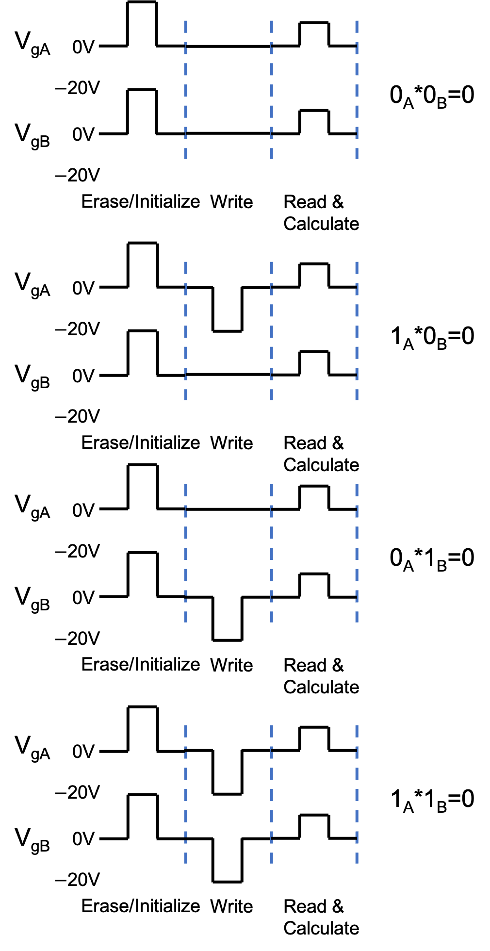
Voltage sequences for erase, write, read, and calculate operations for four AND-gate inputs

An algorithm or a program is a timed sequence of voltage potential \(V(t)\).

\(H(t)=H_{\mathrm{hardware}}+V(t)\)

A quantum algorithm is a time‑dependent Hamiltonian \(H(t)\).

From Reversible Logic to Physical Evolution (I)

\[i\hbar\frac{d}{dt}|\psi(t)\rangle=H(t)|\psi(t)\rangle,\]

\[U(T,0)=\mathcal T\exp\!\left[-\frac{i}{\hbar}\int_0^T H(t)\,dt\right],\]

\[|\psi(T)\rangle=U(T,0)|\psi(0)\rangle.\]
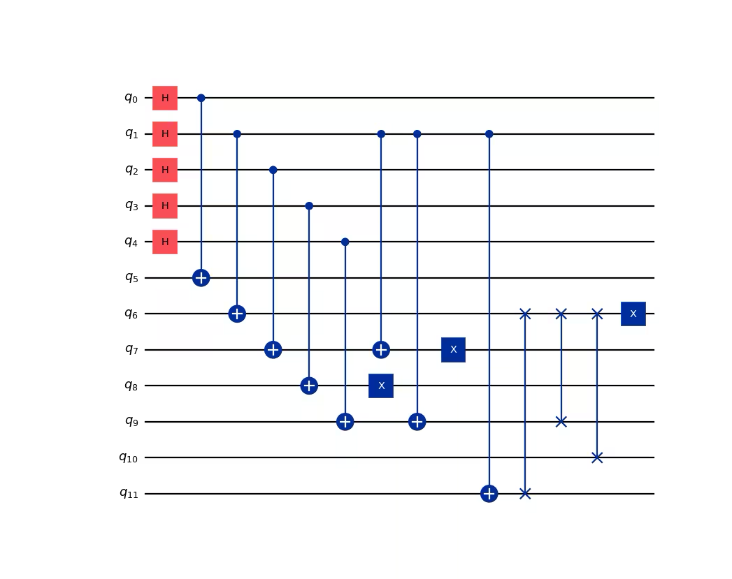
Qiskit example of a twelve-qubit circuit with H, controlled-X, X, and SWAP gates


\[\begin{align*} U(T,0)&\approx \mathcal T\exp\!\left[-\frac{i}{\hbar}\int_{T_n}^T H(t)\,dt\right]*\mathcal T\exp\!\left[-\frac{i}{\hbar}\int_{T_{n-1}}^{T_n} H(t)\,dt\right]*...*\mathcal T\exp\!\left[-\frac{i}{\hbar}\int_0^{T_1} H(t)\,dt\right],\\ &\approx U(T,T_n)*U(T_n,T_{n-1})*...*U(T_1,0) \end{align*}\]

From Reversible Logic to Physical Evolution (II)

\[i\hbar\frac{d}{dt}|\psi(t)\rangle=H(t)|\psi(t)\rangle,\]

\[U(T,0)=\mathcal T\exp\!\left[-\frac{i}{\hbar}\int_0^T H(t)\,dt\right],\]

\[|\psi(T)\rangle=U(T,0)|\psi(0)\rangle.\]


\[\boxed{\text{Reversibility}:\exists U^{-1} \text{ s.t } U*U^{-1}=I}\]

\[U^{-1}(T,0)=U(0,T)=U^\dagger(T,0)=\mathcal T\exp\!\left[\textcolor{red}{+}\frac{i}{\hbar}\int_0^T H(t)\,dt\right]\]

\[\langle \psi(T)|\psi(T)\rangle=\langle \psi(0)|U^\dagger(T,0)* U(T,0)|\psi(T)\rangle=\langle \psi(0)|\psi(0)\rangle=1\]

Qiskit example of a twelve-qubit circuit with H, controlled-X, X, and SWAP gates


\[\begin{align*} U(T,0)&\approx \mathcal T\exp\!\left[-\frac{i}{\hbar}\int_{T_n}^T H(t)\,dt\right]*\mathcal T\exp\!\left[-\frac{i}{\hbar}\int_{T_{n-1}}^{T_n} H(t)\,dt\right]*...*\mathcal T\exp\!\left[-\frac{i}{\hbar}\int_0^{T_1} H(t)\,dt\right],\\ &\approx U(T,T_n)*U(T_n,T_{n-1})*...*U(T_1,0) \end{align*}\]


\[\boxed{\text{Boolean function}\rightarrow\text{reversible embedding}\rightarrow\text{unitary}\rightarrow H(t).}\]

Information Erasure Makes Logic Irreversible

A gate is reversible only when its output identifies one unique input.
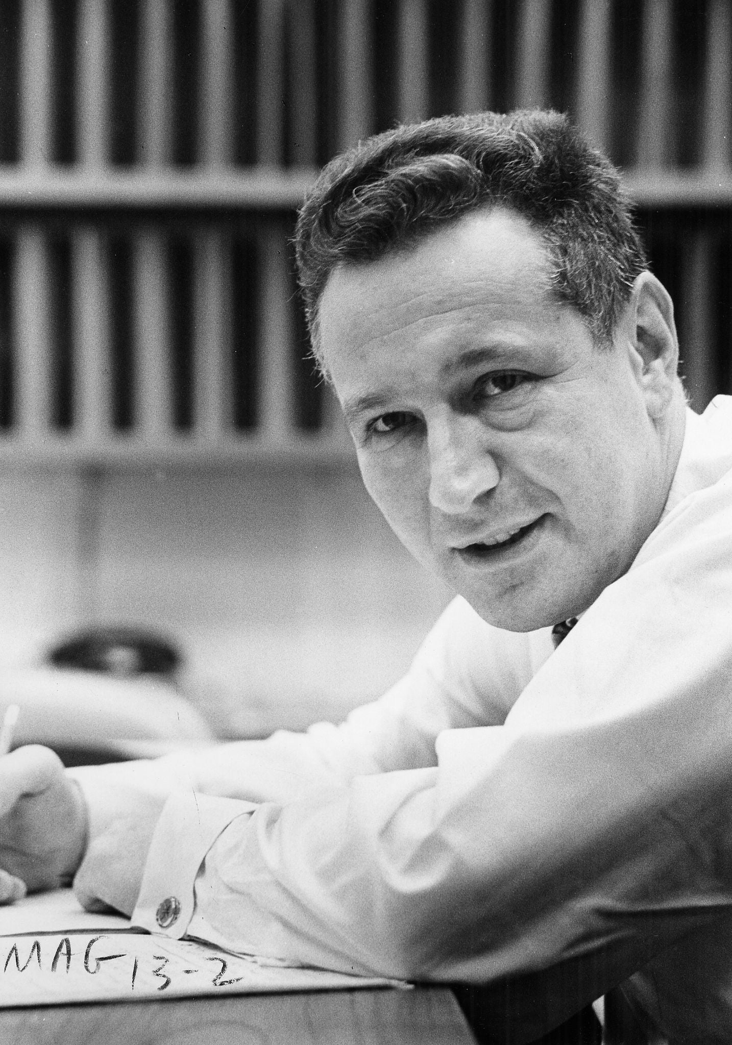
Portrait of Rolf Landauer
Rolf Landauer

Erasing one unbiased bit requires the environment to receive at least

\[\Delta S_{\mathrm{env}}\ge k_B\ln2\]

\[Q_{\min}\ge k_BT\ln2\]

Half-adder circuit
Half-adder truth table ordered as Carry then Sum

Half adder: \(01\) and \(10\) both produce \((\mathrm{Carry},\mathrm{Sum})=(0,1)\).

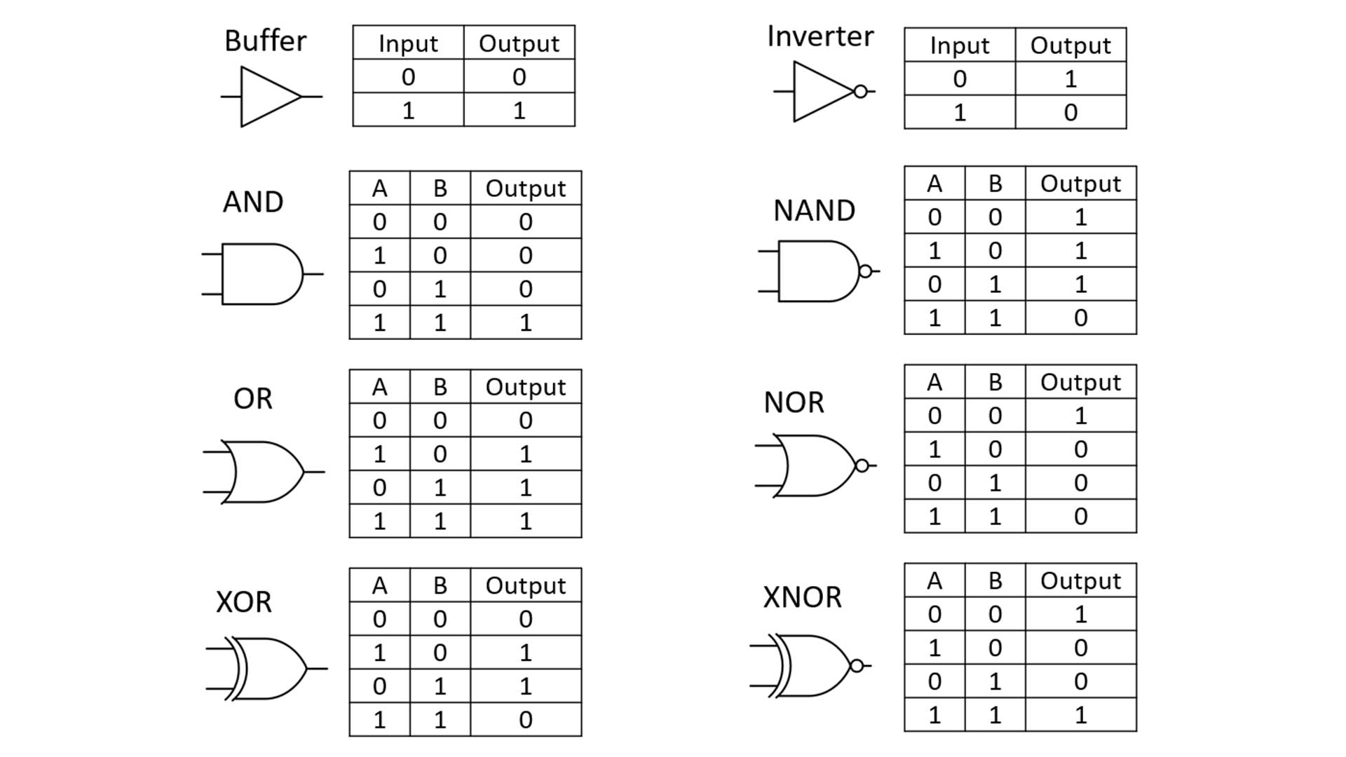
Logic-gate symbols and truth tables; Buffer and NOT are one-to-one while the two-input gates shown are many-to-one × × × × × ×
Buffer and NOT(Invertor) are one-to-one. The crossed two-input gates are many-to-one.

Source: Landauer (1961).

Controlled Gates Preserve Their Inputs (I)
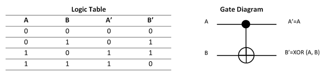
CNOT truth table and gate diagram
CNOT: \((A,B)\mapsto(A,\,B\oplus A)\) — the control \(A\) is preserved.

Controlled Gates Preserve Their Inputs (II)
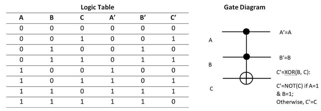
CNOT truth table and gate diagram
CNOT: \((A,B)\mapsto(A,\,B\oplus A)\) — the control \(A\) is preserved.
Toffoli gate truth table and gate diagram
Toffoli / CCNOT: \((A,B,C)\mapsto(A,\,B,\,C\oplus AB)\) — both controls are preserved.

A Reversible Half Adder Keeps Enough Information

Conventional half-adder circuit

Conventional: information is lost

A B Carry Sum
0 0 0 0
0 1 0 1
1 0 0 1
1 1 1 0

01 and 10 both give (Carry, Sum) = (0, 1).
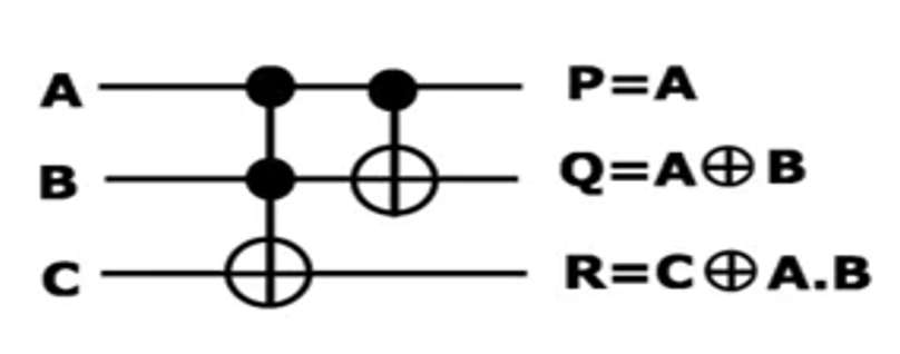
Reversible half-adder circuit with outputs P equals A, Q equals A XOR B, and R equals C XOR AB

Reversible embedding: retain one input

A B C P R = Carry Q = Sum
0 0 0 0 0 0
0 1 0 0 0 1
1 0 0 1 0 1
1 1 0 1 1 0

With C = 0, P = A preserves the input, so 01 and 10 remain distinct.

How we encode algorithm into QUANTUM physical evolution?

Pauli Matrices and Bloch Sphere

From Reversible Logic to Physical Evolution

\[i\hbar\frac{d}{dt}|\psi(t)\rangle=H(t)|\psi(t)\rangle,\]

\[U(T,0)=\mathcal T\exp\!\left[-\frac{i}{\hbar}\int_0^T H(t)\,dt\right],\]

\[|\psi(T)\rangle=U(T,0)|\psi(0)\rangle.\]


\[\boxed{\text{Reversibility}:\exists U^{-1} \text{ s.t } U*U^{-1}=I}\]

\[U^{-1}(T,0)=U(0,T)=U^\dagger(T,0)=\mathcal T\exp\!\left[\textcolor{red}{+}\frac{i}{\hbar}\int_0^T H(t)\,dt\right]\]

\[\langle \psi(T)|\psi(T)\rangle=\langle \psi(0)|U^\dagger(T,0)* U(T,0)|\psi(T)\rangle=\langle \psi(0)|\psi(0)\rangle=1\]

Qiskit example of a twelve-qubit circuit with H, controlled-X, X, and SWAP gates


\[\begin{align*} U(T,0)&\approx \mathcal T\exp\!\left[-\frac{i}{\hbar}\int_{T_n}^T H(t)\,dt\right]*\mathcal T\exp\!\left[-\frac{i}{\hbar}\int_{T_{n-1}}^{T_n} H(t)\,dt\right]*...*\mathcal T\exp\!\left[-\frac{i}{\hbar}\int_0^{T_1} H(t)\,dt\right],\\ &\approx U(T,T_n)*U(T_n,T_{n-1})*...*U(T_1,0) \end{align*}\]


\[\boxed{\text{Boolean function}\rightarrow\text{reversible embedding}\rightarrow\text{unitary}\rightarrow H(t).}\]

Unitary time evolution

\[U(T,0)=\mathcal T\exp\!\left[-\frac{i}{\hbar}\int_0^T H(t)\,dt\right],\]

\[|\psi(T)\rangle=U(T,0)|\psi(0)\rangle.\]
The Hamiltonian \(H\) is Hermitian, so \(U^\dagger(t)U(t)=I\) and total probability remains one.

The time evolution of 2-state system:

\[ \begin{align*} i\hbar \partial_t |\psi \rangle &= H |\psi_\rangle \\ i\hbar \partial_t \begin{pmatrix} \psi_0\\ \psi_1 \end{pmatrix} &=\begin{pmatrix} H_{00}&H;_{01}\\ H_{10}&H;_{11} \end{pmatrix} \begin{pmatrix} \psi_0\\ \psi_1 \end{pmatrix} =\begin{pmatrix} h_a&h;_x-ih_y\\ h_x+ih_y&h;_b \end{pmatrix} \begin{pmatrix} \psi_0\\ \psi_1 \end{pmatrix} \end{align*} \]
\[\qquad a,b,x,y\in\mathbb R\]

Four independent real parameters specify the generator.

Unitary time evolution

\[U(T,0)=\mathcal T\exp\!\left[-\frac{i}{\hbar}\int_0^T H(t)\,dt\right],\]

\[|\psi(T)\rangle=U(T,0)|\psi(0)\rangle.\]
The Hamiltonian \(H\) is Hermitian, so \(U^\dagger(t)U(t)=I\) and total probability remains one.

The time evolution of 2-state system:

\[ \begin{align*} i\hbar \partial_t |\psi \rangle &= H |\psi_\rangle \\ i\hbar \partial_t \begin{pmatrix} \psi_0\\ \psi_1 \end{pmatrix} &=\begin{pmatrix} H_{00}&H;_{01}\\ H_{10}&H;_{11} \end{pmatrix} \begin{pmatrix} \psi_0\\ \psi_1 \end{pmatrix} =\begin{pmatrix} h_a&h;_x-ih_y\\ h_x+ih_y&h;_b \end{pmatrix} \begin{pmatrix} \psi_0\\ \psi_1 \end{pmatrix} \end{align*} \]
\[\qquad a,b,x,y\in\mathbb R\]

Four independent real parameters specify the generator.

Separate the trace

\[ c=\frac{h_a+h_b}{2}, \ h_z=\frac{h_a-h_b}{2} \]

Identity part and traceless part

\[ \begin{align*} H=\begin{pmatrix} c+h_z&h;_x-ih_y\\ h_x+ih_y&c-h;_z \end{pmatrix} &= c\begin{pmatrix} 1&0\\ 0&1 \end{pmatrix} +h_x\begin{pmatrix} 0&1\\ 1&0 \end{pmatrix} +h_y\begin{pmatrix} 0&-i\\ i&0 \end{pmatrix} +h_z\begin{pmatrix} 1&0\\ 0&-1 \end{pmatrix} \\&\equiv cI + \underbracket{h_x\sigma_x +h_y\sigma_y +h_z\sigma_z}_{H'}, \quad \sigma_i \text{ :Pauli matrices} \end{align*} \]

Unitary time evolution

\[U(T,0)=\mathcal T\exp\!\left[-\frac{i}{\hbar}\int_0^T H(t)\,dt\right],\]

\[|\psi(T)\rangle=U(T,0)|\psi(0)\rangle.\]
The Hamiltonian \(H\) is Hermitian, so \(U^\dagger(t)U(t)=I\) and total probability remains one.

The time evolution of 2-state system:

\[ \begin{align*} i\hbar \partial_t |\psi \rangle &= H |\psi_\rangle \\ i\hbar \partial_t \begin{pmatrix} \psi_0\\ \psi_1 \end{pmatrix} &=\begin{pmatrix} H_{00}&H;_{01}\\ H_{10}&H;_{11} \end{pmatrix} \begin{pmatrix} \psi_0\\ \psi_1 \end{pmatrix} =\begin{pmatrix} h_a&h;_x-ih_y\\ h_x+ih_y&h;_b \end{pmatrix} \begin{pmatrix} \psi_0\\ \psi_1 \end{pmatrix} \end{align*} \]
\[\qquad a,b,x,y\in\mathbb R\]

Four independent real parameters specify the generator.

Separate the trace

\[ c=\frac{h_a+h_b}{2}, \ h_z=\frac{h_a-h_b}{2} \]

Identity part and traceless part

\[ \begin{align*} H=\begin{pmatrix} c+h_z&h;_x-ih_y\\ h_x+ih_y&c-h;_z \end{pmatrix} &= c\begin{pmatrix} 1&0\\ 0&1 \end{pmatrix} +h_x\begin{pmatrix} 0&1\\ 1&0 \end{pmatrix} +h_y\begin{pmatrix} 0&-i\\ i&0 \end{pmatrix} +h_z\begin{pmatrix} 1&0\\ 0&-1 \end{pmatrix} \\&\equiv cI + \underbracket{h_x\sigma_x +h_y\sigma_y +h_z\sigma_z}_{H'}, \quad \sigma_i \text{ :Pauli matrices} \end{align*} \]

\[ e^{-itH}=e^{-it(cI+H')}=e^{-itc}e^{-itH'} \]

The factor \(e^{-itc}\) is a global phase. Observable state evolution therefore comes from \(H'\).

Properties of the Pauli Matrices (I)

\[ \sigma_x=\begin{pmatrix}0&1\\1&0\end{pmatrix},\qquad \sigma_y=\begin{pmatrix}0&-i\\i&0\end{pmatrix},\qquad \sigma_z=\begin{pmatrix}1&0\\0&-1\end{pmatrix}. \]

\[ \boxed{\sigma_i\sigma_j=\delta_{ij}I+i \epsilon_{ijk}\sigma_k} \]

\[ \sigma_i \sigma_j=- \sigma_j \sigma_i=i \epsilon_{ijk}\sigma_k , \qquad \sigma_x \sigma_x =\sigma_y \sigma_y =\sigma_z \sigma_z= I, \qquad \operatorname{Tr} (\sigma_i)=0. \]

Properties of the Pauli Matrices (II)

\[ \sigma_x=\begin{pmatrix}0&1\\1&0\end{pmatrix},\qquad \sigma_y=\begin{pmatrix}0&-i\\i&0\end{pmatrix},\qquad \sigma_z=\begin{pmatrix}1&0\\0&-1\end{pmatrix}. \]

\[ \boxed{\sigma_i\sigma_j=\delta_{ij}I+i \epsilon_{ijk}\sigma_k} \]

\[ \sigma_i \sigma_j=- \sigma_j \sigma_i=i \epsilon_{ijk}\sigma_k , \qquad \sigma_x \sigma_x =\sigma_y \sigma_y =\sigma_z \sigma_z= I, \qquad \operatorname{Tr} (\sigma_i)=0. \]

\[ \begin{align*} H&= cI + h_x\sigma_x +h_y\sigma_y +h_z\sigma_z \end{align*} \]

\[ \begin{align*} h_i =\frac{1}{2} \operatorname{Tr}(H\sigma_i) \end{align*} \]

For example, \[ \begin{align*} h_x = \frac{1}{2}\operatorname{Tr}(H\sigma_x) &= \frac{1}{2}\operatorname{Tr}\left[\left(cI + h_x\sigma_x +h_y\sigma_y +h_z\sigma_z\right)\sigma_x\right]\\ &=\frac{1}{2} \operatorname{Tr}\left(c \sigma_x + h_x\sigma_x \sigma_x +h_y\sigma_y \sigma_x +h_z\sigma_z \sigma_x\right)\\ &=\frac{1}{2} \operatorname{Tr}\left(c \sigma_x + h_x I -i h_y\sigma_z + i h_z\sigma_y \right) \end{align*} \]

Properties of the Pauli Matrices (III)

\[ \sigma_x=\begin{pmatrix}0&1\\1&0\end{pmatrix},\qquad \sigma_y=\begin{pmatrix}0&-i\\i&0\end{pmatrix},\qquad \sigma_z=\begin{pmatrix}1&0\\0&-1\end{pmatrix}. \]

\[ \boxed{\sigma_i\sigma_j=\delta_{ij}I+i \epsilon_{ijk}\sigma_k} \]

\[ \sigma_i \sigma_j=- \sigma_j \sigma_i=i \epsilon_{ijk}\sigma_k , \qquad \sigma_x \sigma_x =\sigma_y \sigma_y =\sigma_z \sigma_z= I, \qquad \operatorname{Tr} (\sigma_i)=0. \]

Each Pauli matrix

\[ \sigma_i^\dagger=\sigma_i,\qquad \sigma_i^2=I,\qquad \sigma_i^{-1}=\sigma_i \]

\[ \operatorname{spec}(\sigma_i)=\{+1,-1\}. \]

Pauli-\(Z\) gate and Z-axis \(Z\equiv \sigma_z, \quad \left\{ \begin{array}{c} Z|0\rangle=+|0\rangle \\ Z|1\rangle=-|1\rangle \end{array} \right.\)
Pauli-\(X\) gate and X-axis \( X\equiv \sigma_x, \ \left\{ \begin{array}{c} X|+\rangle=+|+\rangle \\ X|-\rangle=-|-\rangle \end{array} \right. , \ |\pm\rangle=\tfrac{|0\rangle\pm|1\rangle}{\sqrt2} \)
Pauli-\(Y\) gate and Y-axis \(Y\equiv \sigma_y, \ \left\{ \begin{array}{c} Y|i\rangle=+|i\rangle \\ Y|-i\rangle=-|-i\rangle \end{array} \right. , \ |\pm i\rangle=\tfrac{|0\rangle\pm i|1\rangle}{\sqrt2} \)

Visualizing a Qubit State on the Bloch Sphere

Bloch sphere with the six Pauli eigenstates and a general state labelled by theta and phi

For any two state system with orthonormal basis \(|a \rangle, \ |b \rangle\) \[|\psi\rangle = c_0 |a \rangle + c_1 |b \rangle,\quad c_k=|c_k|e^{i\phi_k}\in \mathbb{C},\quad \langle a|b \rangle=0\] \[\left\{ \begin{array}{c} \langle \psi|\psi \rangle=1 \to |c_0|^2+|c_1|^2=1 \\ \text{unobservable global phase }\phi_0 \end{array} \right.\] \[|\psi(\theta,\phi)\rangle =\cos\!\left(\frac{\theta}{2}\right)|a\rangle +e^{i\phi}\sin\!\left(\frac{\theta}{2}\right)|b\rangle \]

\(0\leq\theta\leq\pi,\qquad 0\leq\phi< 2\pi\)

We normally choose \(|0 \rangle, \ |1 \rangle\) as our orthonormal basis \(|0 \rangle=\left( \begin{array}{c} 1 \\ 0 \end{array} \right), \ |1 \rangle =\left( \begin{array}{c} 0 \\ 1 \end{array} \right), \ |\psi \rangle =\left( \begin{array}{c} \cos\!\left(\frac{\theta}{2}\right) \\ e^{i\phi}\sin\!\left(\frac{\theta}{2}\right) \end{array} \right) \)

\[|\psi\rangle = c_0 |0 \rangle + c_1 |1 \rangle, c_k=|c_k|e^{i\phi_k}\in \mathbb{C}\]

\[|c_0|^2+|c_1|^2=1 \to \left\{ \begin{array}{c} |c_0|\equiv \cos \left( \frac{\theta}{2} \right) \\ |c_1|\equiv \sin \left( \frac{\theta}{2} \right) \end{array} \right.\]

\[|\psi\rangle = \cos \left( \frac{\theta}{2} \right)e^{i\phi_0}|0\rangle +\sin \left( \frac{\theta}{2} \right)e^{i\phi_1}|1\rangle\]

\[=e^{i\phi_0}\left[ \cos \left( \frac{\theta}{2} \right)|0\rangle +\sin \left( \frac{\theta}{2} \right)e^{i(\phi_1-\phi_0)}|1\rangle \right]\]

\[\equiv e^{i\phi_0}\left[ \cos \left( \frac{\theta}{2} \right)|0\rangle +\sin \left( \frac{\theta}{2} \right)e^{i\phi}|1\rangle \right] =e^{i\phi_0}\begin{pmatrix} \cos(\theta/2)\\ e^{i\phi}\sin(\theta/2) \end{pmatrix}\]

Density matrix \(\rho\):

\[\rho\equiv|\psi\rangle\langle\psi| =e^{i\phi_0}\begin{pmatrix} \cos(\theta/2)\\ e^{i\phi}\sin(\theta/2) \end{pmatrix} \otimes e^{-i\phi_0}\begin{pmatrix} \cos(\theta/2)&e;^{-i\phi}\sin(\theta/2) \end{pmatrix}\]

\[=\begin{pmatrix} \cos^2(\theta/2)&e;^{-i\phi}\sin(\theta/2)\cos(\theta/2)\\ e^{i\phi}\sin(\theta/2)\cos(\theta/2)&\sin^2(\theta/2) \end{pmatrix}\]

\[=\frac12\begin{pmatrix} 1+\cos\theta&e;^{-i\phi}\sin\theta\\ e^{i\phi}\sin\theta&1-\cos\theta \end{pmatrix}\]

Bloch sphere with the six Pauli eigenstates and a general state labelled by theta and phi

\[|\psi\rangle = e^{i\phi_0}\left[ \cos \left( \frac{\theta}{2} \right) \ |0 \rangle + \sin \left( \frac{\theta}{2} \right) \ e^{i\phi} |1 \rangle \right] \]

Density matrix \(\rho\): \[ \rho \equiv |\psi \rangle \langle \psi | = \frac{1}{2}\begin{pmatrix} 1+\cos \theta & e^{-i\phi}\sin \theta \\ e^{i\phi}\sin \theta & 1-\cos \theta \end{pmatrix} \]

\[ =\frac{1}{2}\begin{pmatrix} 1+\cos \theta & \cos \phi \sin \theta-i\sin \phi \sin \theta \\ \cos \phi \sin \theta+i\sin \phi \sin \theta & 1-\cos \theta \end{pmatrix} \]

\[ =\frac{1}{2}\left[ \begin{pmatrix}1&0\\0&1\end{pmatrix} +\cos \phi \sin \theta\begin{pmatrix}0&1\\1&0\end{pmatrix} +\sin \phi \sin \theta\begin{pmatrix}0&-i\\i&0\end{pmatrix} +\cos \theta\begin{pmatrix}1&0\\0&-1\end{pmatrix} \right] \]

\[ \equiv\frac{1}{2}\left[ I+r_x\sigma_x+r_y\sigma_y+r_z\sigma_z \right] \]

Bloch sphere with the six Pauli eigenstates and a general state labelled by theta and phi

\[ r_i=\operatorname{Tr}(\rho\sigma_i) \]

For example, \[ \begin{aligned} r_x=\operatorname{Tr}(\rho\sigma_x) &=\frac{1}{2}\operatorname{Tr}\left[\left(cI+ r_x\sigma_x+r_y\sigma_y+r_z\sigma_z\right)\sigma_x\right] \end{aligned} \]

\[ \begin{aligned} &=\frac{1}{2}\operatorname{Tr}\left(c \sigma_x+ r_x\sigma_x\sigma_x+r_y\sigma_y\sigma_x+r_z\sigma_z\sigma_x\right) \end{aligned} \]

\[ \begin{aligned} &=\frac{1}{2}\operatorname{Tr}\left(c \sigma_x+ r_x I-ir_y\sigma_z+ir_z\sigma_y\right) \end{aligned} \]

\[|\psi\rangle = e^{i\phi_0}\left[ \cos \left( \frac{\theta}{2} \right) \ |0 \rangle + \sin \left( \frac{\theta}{2} \right) \ e^{i\phi} |1 \rangle \right] \]

Density matrix \(\rho\): \[\begin{align*} \rho \equiv |\psi \rangle \langle \psi | &=\frac{1}{2}\left[ I +\cos \phi \sin \theta \ \sigma_x +\sin \phi \sin \theta \ \sigma_y +\cos \theta \ \sigma_z \right]\\ &= \frac{1}{2}\left[ I + r_x \sigma_x + r_y \sigma_y + r_z \sigma_z \right]\end{align*}\]
\[\begin{align*} r_i &=\operatorname{Tr}(\rho\sigma_i) \end{align*}\]

Bloch sphere with the six Pauli eigenstates and a general state labelled by theta and phi

Caution:
(1) \(|\psi\rangle\neq r_x|+\rangle+r_y|i\rangle+r_z|0\rangle\).

(2) \(|1\rangle\neq -|0\rangle,\ |-\rangle\neq-|+\rangle,\ |-i\rangle\neq -|i\rangle\).

(3) \(-|0\rangle=e^{-i\pi}|0\rangle\) differs from \(|0\rangle\) by a global phase.

Single-Qubit Rotation Operators

\[ \begin{align*} H&= cI + h_x\sigma_x +h_y\sigma_y +h_z\sigma_z \end{align*} \]

\[ U(t)=e^{-itH}=e^{-it(cI +h_x\sigma_x +h_y\sigma_y +h_z\sigma_z)} \]

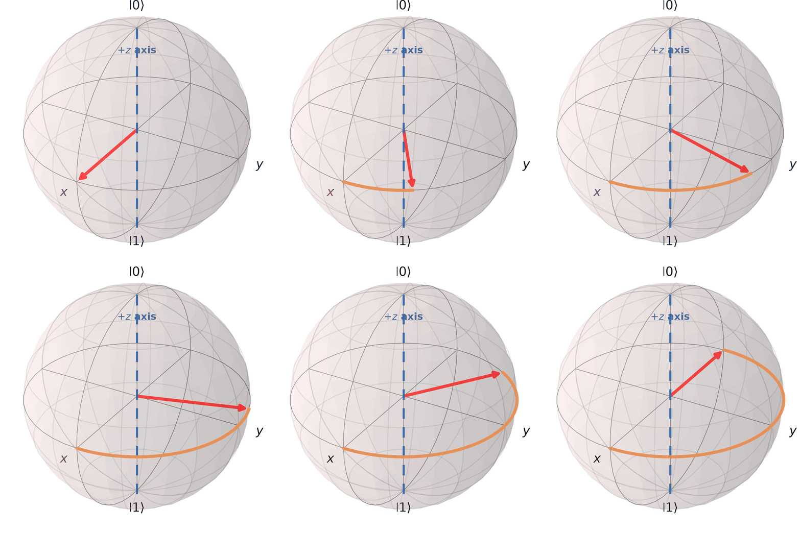
\(R_x(\alpha)\equiv e^{\left(-i\frac{\alpha}{2}\sigma_x\right)}\)

\(R_y(\alpha)\equiv e^{\left(-i\frac{\alpha}{2}\sigma_y\right)}\)

\(R_z(\alpha)\equiv e^{\left(-i\frac{\alpha}{2}\sigma_z\right)}\)

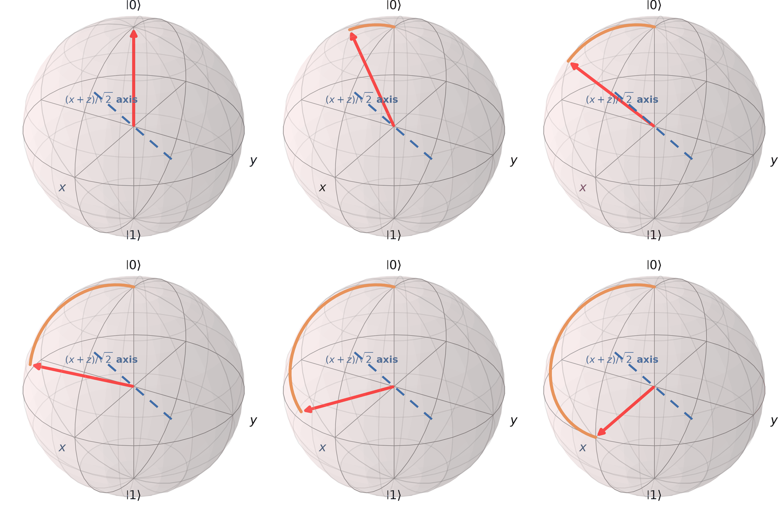
\(R_{\hat{\mathbf n}_H}(\alpha)\)

\(\hat{\mathbf n}_H=(\hat{\mathbf x}+\hat{\mathbf z})/\sqrt2\)
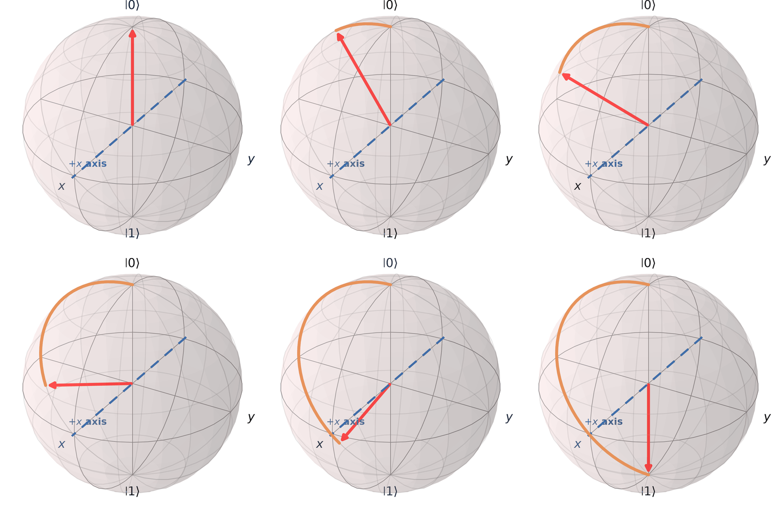
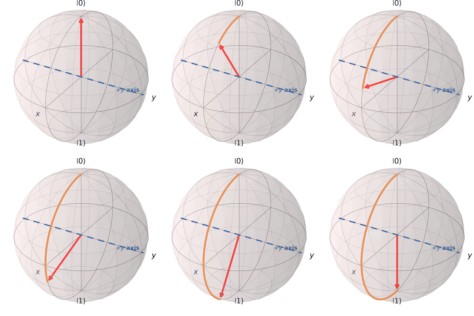
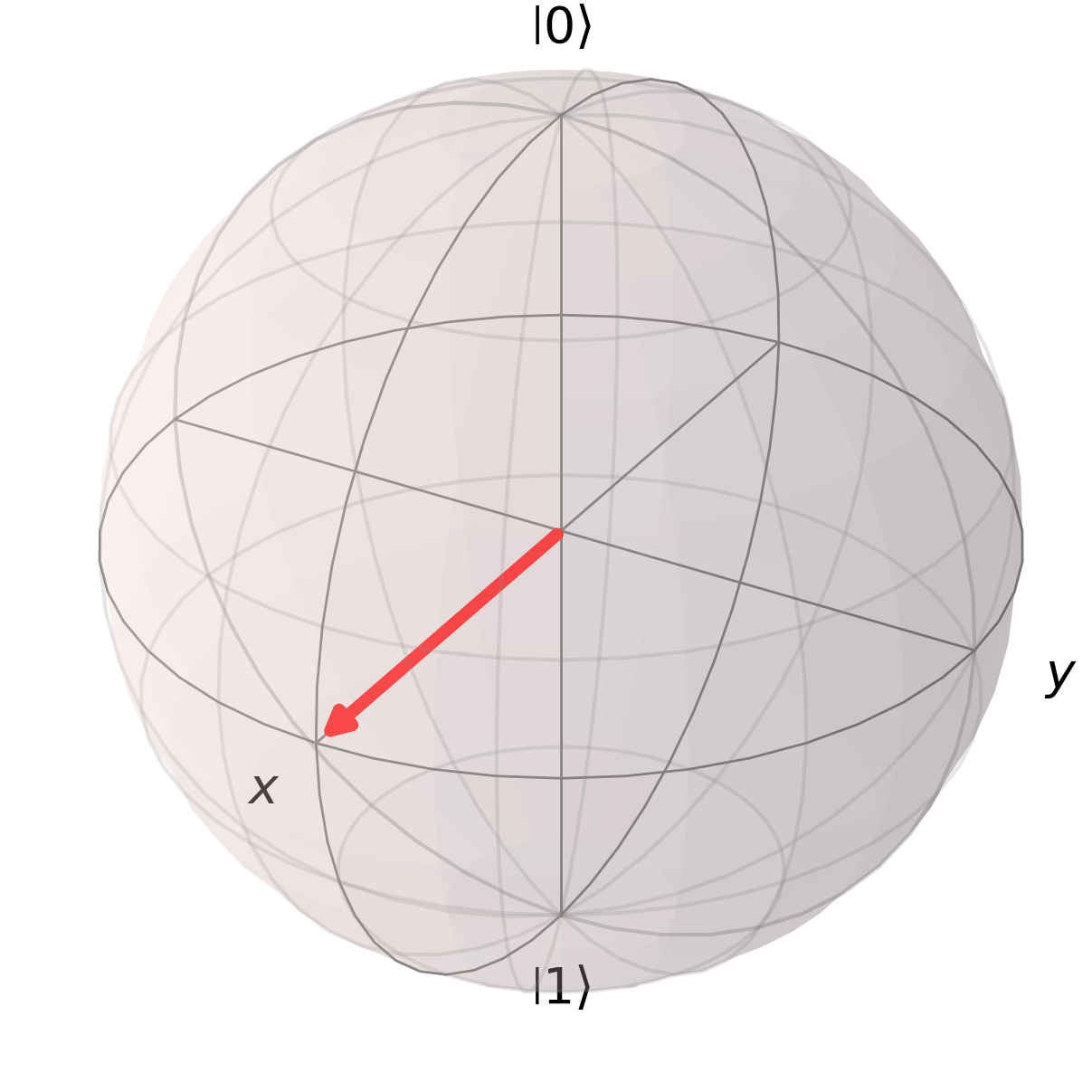
Bloch-sphere animation of a pi rotation about the positive x axis
Bloch-sphere animation of a pi rotation about the positive y axis
Bloch-sphere animation of a pi rotation about the positive z axis
Bloch-sphere animation of a pi rotation about the x plus z axis

Evolution of a Qubit State

State vector

\[|\psi'\rangle=U|\psi\rangle\]

→

Density matrix

\[\boxed{\rho'=U\rho U^\dagger}\]

→

Bloch coordinates

\[\rho'=\frac12\left(I+\mathbf r'\!\cdot\!\boldsymbol{\sigma}\right)\]

Since \(r_i'=\operatorname{Tr}(\rho'\sigma_i)\), cyclicity of the trace gives

\[ \boxed{ r_i'=\operatorname{Tr}(U\rho U^\dagger\sigma_i) =\operatorname{Tr}\!\left(\rho\,U^\dagger\sigma_iU\right)}. \]

Evolution of a Qubit State

State vector

\[|\psi'\rangle=U|\psi\rangle\]

→

Density matrix

\[\boxed{\rho'=U\rho U^\dagger}\]

→

Bloch coordinates

\[\rho'=\frac12\left(I+\mathbf r'\!\cdot\!\boldsymbol{\sigma}\right)\]

Since \(r_i'=\operatorname{Tr}(\rho'\sigma_i)\), cyclicity of the trace gives

\[ \boxed{ r_i'=\operatorname{Tr}(U\rho U^\dagger\sigma_i) =\operatorname{Tr}\!\left(\rho\,U^\dagger\sigma_iU\right)}. \]

For example, \(U_x=R_x(\alpha)= e^{\left(-i\frac{\alpha}{2}\sigma_x\right)}\)

State vector

\[|\psi'\rangle=U_x|\psi\rangle\]

→

Density matrix

\[\boxed{\rho'=U_x\rho U^\dagger_x}\]

→

Bloch coordinates

\[\rho'=\frac12\left(I+\mathbf r'\!\cdot\!\boldsymbol{\sigma}\right)\]

Expanding \(e^{-i\alpha\sigma_x/2}\) Term by Term

Split into \(\cos\) and \(i\sin\)

\[ e^{-i\frac\alpha2\sigma_x} =\cos\!\left(\frac\alpha2\sigma_x\right) -i\sin\!\left(\frac\alpha2\sigma_x\right) \]

Taylor expand each

\[ \begin{aligned} \cos\!\left(\frac\alpha2\sigma_x\right) &=I -\frac{1}{2!} \left(\frac\alpha2\sigma_x\right)^{2} +\frac{1}{4!} \left(\frac\alpha2\sigma_x\right)^{4}-... =I -\frac{1}{2!} \left(\frac\alpha2\right)^{2}\left(\sigma_x\right)^{2} +\frac{1}{4!} \left(\frac\alpha2\right)^{4}\left(\sigma_x\right)^{4}-... ,\\[2pt] \sin\!\left(\frac\alpha2\sigma_x\right) &=\left(\frac\alpha2\sigma_x\right) -\frac{1}{3!} \left(\frac\alpha2\sigma_x\right)^{3}+... =\left(\frac\alpha2\right)\sigma_x -\frac{1}{3!} \left(\frac\alpha2\right)^{3}\left(\sigma_x\right)^{3}+... \end{aligned} \]

Collapse the operators

\[ \sigma_x^{2}=I \quad\Longrightarrow\quad \sigma_x^{2m}=I, \qquad \sigma_x^{2m+1}=\sigma_x. \]

\[ \begin{aligned} \cos\!\left(\frac\alpha2\sigma_x\right) &=I -\frac{1}{2!} \left(\frac\alpha2\right)^{2}I +\frac{1}{4!} \left(\frac\alpha2\right)^{4}I-... =\cos\frac\alpha2\,I,\\[2pt] \sin\!\left(\frac\alpha2\sigma_x\right) &=\left(\frac\alpha2\right)\sigma_x -\frac{1}{3!} \left(\frac\alpha2\right)^{3}\sigma_x+... =\sin\frac\alpha2\,\sigma_x. \end{aligned} \]

Tidy up

\[ \boxed{\;e^{-i\frac\alpha2\sigma_x} =\cos\frac\alpha2\,I-i\sin\frac\alpha2\,\sigma_x\;} \]

Deriving the \(x\)-Axis Bloch Rotation

\[ \rho=\frac12\left(I+r_x\sigma_x+r_y\sigma_y+r_z\sigma_z\right), \qquad U_x(\alpha)=\cos\tfrac\alpha2\,I-i\sin\tfrac\alpha2\,\sigma_x, \qquad r_x=\operatorname{Tr}(\rho'\sigma_x) \to r_x'=\operatorname{Tr}(\rho U^\dagger \sigma_x U). \]

\(U_x^\dagger\sigma_xU_x\) \(=\) \(\left(\cos\!\left(\frac{\alpha}{2}\right)I+i\sin\!\left(\frac{\alpha}{2}\right)\sigma_x\right)\sigma_x\left(\cos\!\left(\frac{\alpha}{2}\right)I-i\sin\!\left(\frac{\alpha}{2}\right)\sigma_x\right)\)
\(=\) \(\cos^2\!\left(\frac{\alpha}{2}\right)\sigma_x-i\cos\!\left(\frac{\alpha}{2}\right)\sin\!\left(\frac{\alpha}{2}\right)\sigma_x^2\) \(+i\cos\!\left(\frac{\alpha}{2}\right)\sin\!\left(\frac{\alpha}{2}\right)\sigma_x^2+\sin^2\!\left(\frac{\alpha}{2}\right)\sigma_x^3\)
\(=\) \(\left[\cos^2\!\left(\frac{\alpha}{2}\right)+\sin^2\!\left(\frac{\alpha}{2}\right)\right]\sigma_x\)
\(=\) \(\sigma_x.\)

Read off \(r_x'\)

\(r_x'\) \(=\) \(\operatorname{Tr}(\rho'\sigma_x)\)
\(=\) \(\operatorname{Tr}(U_x\rho U_x^\dagger\sigma_x)\)
\(=\) \(\operatorname{Tr}(\rho U_x^\dagger\sigma_xU_x)\)
\(=\) \(\operatorname{Tr}(\rho\sigma_x)\)
\(=\) \(r_x.\)

Deriving the \(x\)-Axis Bloch Rotation

\[ \rho=\frac12\left(I+r_x\sigma_x+r_y\sigma_y+r_z\sigma_z\right), \qquad U_x(\alpha)=\cos\tfrac\alpha2\,I-i\sin\tfrac\alpha2\,\sigma_x, \qquad r_y=\operatorname{Tr}(\rho'\sigma_y) \to r_y'=\operatorname{Tr}(\rho U^\dagger \sigma_y U). \]

\(\sigma_y\sigma_x=-i\sigma_z,\qquad \sigma_x\sigma_y=i\sigma_z,\qquad \sigma_x\sigma_y\sigma_x=-\sigma_y.\)
\(U_x^\dagger\sigma_yU_x\) \(=\) \(\left(\cos\!\left(\frac{\alpha}{2}\right)I+i\sin\!\left(\frac{\alpha}{2}\right)\sigma_x\right)\sigma_y\left(\cos\!\left(\frac{\alpha}{2}\right)I-i\sin\!\left(\frac{\alpha}{2}\right)\sigma_x\right)\)
\(=\) \(\cos^2\!\left(\frac{\alpha}{2}\right)\sigma_y-i\cos\!\left(\frac{\alpha}{2}\right)\sin\!\left(\frac{\alpha}{2}\right)\sigma_y\sigma_x\) \(+i\cos\!\left(\frac{\alpha}{2}\right)\sin\!\left(\frac{\alpha}{2}\right)\sigma_x\sigma_y+\sin^2\!\left(\frac{\alpha}{2}\right)\sigma_x\sigma_y\sigma_x\)
\(=\) \(\left[\cos^2\!\left(\frac{\alpha}{2}\right)-\sin^2\!\left(\frac{\alpha}{2}\right)\right]\sigma_y -2\cos\!\left(\frac{\alpha}{2}\right)\sin\!\left(\frac{\alpha}{2}\right)\sigma_z\)
\(=\) \(\cos\alpha\,\sigma_y-\sin\alpha\,\sigma_z,\)

Read off \(r_y'\)

\(r_y'\) \(=\) \(\operatorname{Tr}(\rho'\sigma_y)\)
\(=\) \(\operatorname{Tr}(\rho U_x^\dagger\sigma_yU_x)\)
\(=\) \(\operatorname{Tr}\!\left[\rho(\cos\alpha\,\sigma_y-\sin\alpha\,\sigma_z)\right]\)
\(=\) \(\cos\alpha\operatorname{Tr}(\rho\,\sigma_y)-\sin\alpha\operatorname{Tr}(\rho\,\sigma_z)\)
\(=\) \(r_y\cos\alpha-r_z\sin\alpha.\)

Deriving the \(x\)-Axis Bloch Rotation

\[ \rho=\frac12\left(I+r_x\sigma_x+r_y\sigma_y+r_z\sigma_z\right), \qquad U_x(\alpha)=\cos\tfrac\alpha2\,I-i\sin\tfrac\alpha2\,\sigma_x, \qquad r_z=\operatorname{Tr}(\rho'\sigma_z) \to r_z'=\operatorname{Tr}(\rho U^\dagger \sigma_z U). \]

\(\sigma_z\sigma_x=i\sigma_y,\qquad \sigma_x\sigma_z=-i\sigma_y,\qquad \sigma_x\sigma_z\sigma_x=-\sigma_z.\)
\(U_x^\dagger\sigma_zU_x\) \(=\) \(\left(\cos\!\left(\frac{\alpha}{2}\right)I+i\sin\!\left(\frac{\alpha}{2}\right)\sigma_x\right)\sigma_z\left(\cos\!\left(\frac{\alpha}{2}\right)I-i\sin\!\left(\frac{\alpha}{2}\right)\sigma_x\right)\)
\(=\) \(\cos^2\!\left(\frac{\alpha}{2}\right)\sigma_z-i\cos\!\left(\frac{\alpha}{2}\right)\sin\!\left(\frac{\alpha}{2}\right)\sigma_z\sigma_x\) \(+i\cos\!\left(\frac{\alpha}{2}\right)\sin\!\left(\frac{\alpha}{2}\right)\sigma_x\sigma_z+\sin^2\!\left(\frac{\alpha}{2}\right)\sigma_x\sigma_z\sigma_x\)
\(=\) \(2\cos\!\left(\frac{\alpha}{2}\right)\sin\!\left(\frac{\alpha}{2}\right)\sigma_y +\left[\cos^2\!\left(\frac{\alpha}{2}\right)-\sin^2\!\left(\frac{\alpha}{2}\right)\right]\sigma_z\)
\(=\) \(\sin\alpha\,\sigma_y+\cos\alpha\,\sigma_z,\)

Read off \(r_z'\)

\(r_z'\) \(=\) \(\operatorname{Tr}(\rho'\sigma_z)\)
\(=\) \(\operatorname{Tr}(\rho U_x^\dagger\sigma_zU_x)\)
\(=\) \(\operatorname{Tr}\!\left[\rho(\sin\alpha\,\sigma_y+\cos\alpha\,\sigma_z)\right]\)
\(=\) \(\sin\alpha\operatorname{Tr}(\rho\,\sigma_y)+\cos\alpha\operatorname{Tr}(\rho\,\sigma_z)\)
\(=\) \(r_y\sin\alpha+r_z\cos\alpha.\)

Deriving the \(x\)-Axis Bloch Rotation

\[ \rho=\frac12\left(I+r_x\sigma_x+r_y\sigma_y+r_z\sigma_z\right), \qquad U_x(\alpha)=\cos\tfrac\alpha2\,I-i\sin\tfrac\alpha2\,\sigma_x, \qquad r_i=\operatorname{Tr}(\rho'\sigma_i) \to r_i'=\operatorname{Tr}(\rho U^\dagger \sigma_i U). \]

Bloch-sphere animation of a rotation about the positive x axis

Combine the three coordinates

\[ \begin{aligned} r_x'&=r_x,\\ r_y'&=r_y\cos\alpha-r_z\sin\alpha,\\ r_z'&=r_y\sin\alpha+r_z\cos\alpha. \end{aligned} \]

\[ \begin{pmatrix}r_x'\\r_y'\\r_z'\end{pmatrix} = \underbrace{\begin{pmatrix} 1&0&0\\ 0&\cos\alpha&-\sin\alpha\\ 0&\sin\alpha&\cos\alpha \end{pmatrix}}_{R_x(\alpha)} \begin{pmatrix}r_x\\r_y\\r_z\end{pmatrix}. \]

\[ \alpha=\frac\pi2:\qquad |0\rangle\longmapsto\frac{|0\rangle-i|1\rangle}{\sqrt2}=|-i\rangle, \]

\[ \alpha=\pi:\qquad |0\rangle\longmapsto-i|1\rangle\sim|1\rangle. \]

Single-Qubit Reversible Gates

Generated by QuTiP Bloch and Matplotlib FuncAnimation.

\(X(NOT)\)

\(\begin{bmatrix}0&1\\1&0\end{bmatrix}\)


\(|0\rangle\leftrightarrow|1\rangle\)


\(X^2=I\)

\(Y\)

\(\begin{bmatrix}0&-i\\i&0\end{bmatrix}\)


\(|0\rangle\to i|1\rangle\)


\(Y^2=I\)

\(Z\)

\(\begin{bmatrix}1&0\\0&-1\end{bmatrix}\)


\(|0\rangle\to |0\rangle\)

\(|1\rangle\to -|1\rangle=e^{-i\pi}|1\rangle\)

\(Z^2=I\)

\(H \ Hadamard\)

\(\frac1{\sqrt2}\begin{bmatrix}1&1\\1&-1\end{bmatrix}\)


\(|0\rangle\to|+\rangle=\frac{|0\rangle+|1\rangle}{\sqrt{2}}\)


\(H^2=I\)

Labelled Bloch sphere showing the |0>, |1>, |+>, |->, |+i> and |-i> poles and the angles theta and phi

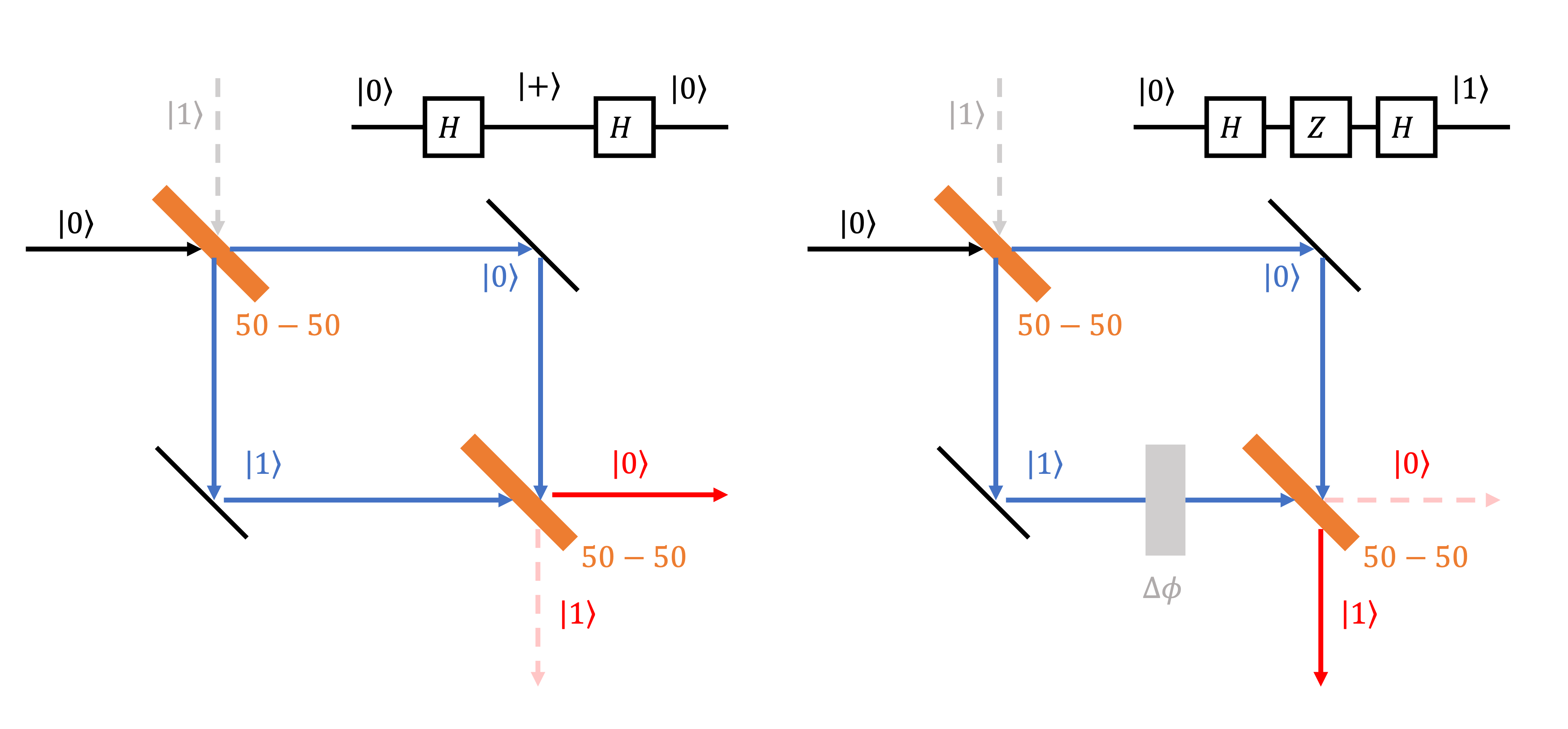
Hadamard \(H\)

Two Mach-Zehnder interferometers: without a phase shift the beams recombine to the |0> port; with a pi phase shift they recombine to the |1> port

\[|0\rangle\xrightarrow{H}\frac{|0\rangle+|1\rangle}{\sqrt2} \xrightarrow{Z}\frac{|0\rangle-|1\rangle}{\sqrt2} \xrightarrow{H}|1\rangle.\]

\[\boxed{\text{superposition}+\text{phase control} +\text{interference}+\text{measurement}.}\]

Question: After the CNOT entangles \(A\) and \(B\), how should the two qubits be drawn?
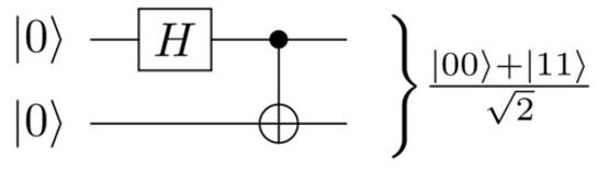
Hadamard followed by CNOT preparing a Bell state

Entanglement:

\(|0_A\rangle |0_B\rangle\xrightarrow{H\otimes I} \left(\frac{|0_A\rangle+|1_A\rangle }{\sqrt2}\right)|0_B\rangle \xrightarrow{\mathrm{CNOT}} \frac{|0_A\rangle |0_B\rangle+|1_A\rangle |1_B\rangle}{\sqrt2}\)

Initial
After \(H_A\)
After CNOT
\(A\)
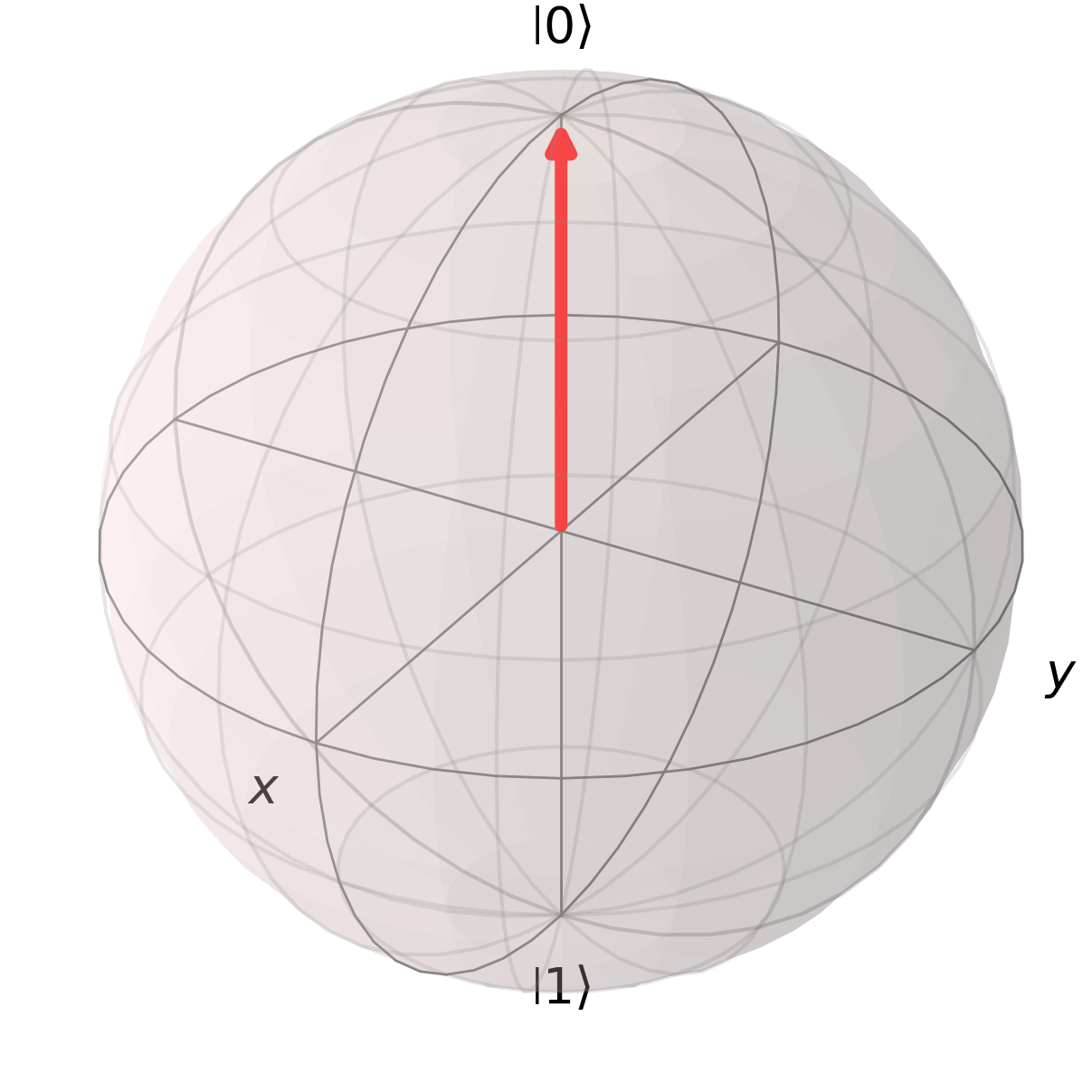
Bloch sphere for qubit A in state zero
\(|0_A\rangle\)
Bloch sphere for qubit A in the plus state
\(|+_A\rangle\)
Empty Bloch sphere for qubit A after CNOT?
\(B\)
Bloch sphere for qubit B in state zero
\(|0_B\rangle\)
Bloch sphere for qubit B after the Hadamard on A
\(|0_B\rangle\)
Empty Bloch sphere for qubit B after CNOT?

Q: Gate-Based vs. Adiabatic Quantum Computing

Gate-Based / Circuit Model

Qiskit example of a twelve-qubit circuit with H, controlled-X, X, and SWAP gates
Google Quantum AI logo IBM Quantum logo Rigetti Computing logo IQM Quantum Computers logo Fujitsu logo Amazon Web Services logo SEEQC logo Alice and Bob logo
Direct figure · IBM Quantum, Qiskit Circuit documentation

Adiabatic Evolution / Quantum Annealing
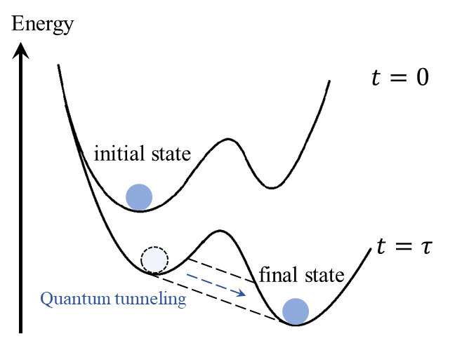
Published diagram of quantum adiabatic evolution from an initial state to a final ground state through a changing energy landscape
D-Wave Quantum logo
Direct figure · Chen et al., Fig. 8 via ResearchGate · CC BY-NC-ND 4.0

Thank you!

Hadamard + CCNOT Is Computationally Universal

CCNOT

\[ |a,b,c\rangle\longmapsto|a,b,c\oplus ab\rangle \]

Reversible Boolean control

+

Hadamard

\[ H|0\rangle=|+\rangle, \qquad H|1\rangle=|-\rangle \]

Basis change and interference

Together they approximate any real quantum evolution to arbitrary accuracy.

Where do the complex amplitudes go?

\(H\) and CCNOT only ever produce real numbers. So split each amplitude into its real and imaginary parts and let one extra qubit, \(\mathrm{RI}\), record which part you are looking at:

\[ \sum_x(a_x+i b_x)|x\rangle \longmapsto \sum_x\Bigl(a_x|x\rangle|0\rangle_{\mathrm{RI}} +b_x|x\rangle|1\rangle_{\mathrm{RI}}\Bigr) \]

\(|0\rangle_{\mathrm{RI}}\) tags the real part \(a_x\), \(|1\rangle_{\mathrm{RI}}\) tags the imaginary part \(b_x\) — so a complex circuit runs entirely on real gates.

Computationally universal, not strictly universal: \(H\) and CCNOT are real matrices; the extra encoding qubit represents complex amplitudes.

Sources: Shi (2003) · Aharonov (2003).

Universal Gate Set

A universal gate set can express every Boolean function.

  • \(\{\mathrm{AND},\mathrm{NOT}\}\) is universal.
  • \(\{\mathrm{OR},\mathrm{NOT}\}\) is universal.
  • \(\{\mathrm{NAND}\}\) alone is universal.
  • \(\{\mathrm{NOR}\}\) alone is universal.
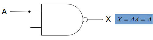
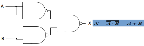
NOT A NOT operation constructed from one NAND gate with its inputs tied together
AND An AND operation constructed from two NAND gates
OR An OR operation constructed from three NAND gates using De Morgan's law

Because NAND reproduces NOT, AND, and OR, NAND alone can generate every Boolean circuit.

Figures: CUNY OpenLab, Lab 05 · CC BY-NC-SA 3.0 · resized.

NAND from a CCNOT Gate

a b c = 1 a b c′ = NAND(a,b)

\[ T(a,b,1)=(a,b,1\oplus ab)=(a,b,\neg(ab)) \]

The controls \(a\) and \(b\) pass through unchanged. The prepared target carries the NAND output.

Truth-table check

\(a\) \(b\) \(c=1\) \(c'=1\oplus ab=\operatorname{NAND}(a,b)\)
0011
0111
1011
1110

The target is 1 except when both controls are 1, exactly the NAND truth table.

CCNOT with a target initialized to \(1\)
→
NAND
→
Any Boolean circuit
CCNOT is universal for classical reversible computation when initialized ancillas and temporary work bits are allowed.

Sources: Toffoli, Reversible Computing (1980) · Morita, Theorem 2.1 (2008).

What Can a Machine Compute?

Computability and Complexity

Does a Quantum Computer Compute More Things?

Computability

Essentially the same

A function \(f\) is computable if one finite algorithm returns the correct \(f(x)\) and halts for every valid input \(x\).

Quantum computers do not cross this boundary: classical and quantum models compute the same computable functions.

Computational complexity

Potentially very different

For an algorithm that halts, complexity asks how the required resources grow as the input size \(n\) increases.

Space complexity  ·  Time complexity
Quantum simulation

Direct dense classical state: \(2^n\) complex amplitudes.
Quantum register: \(n\) qubits represent the state.

Factoring — Shor

Classical: best known general algorithms are sub-exponential.
Quantum: Shor's algorithm runs in polynomial time.

Same computable functions; potentially different resource scaling.

Feynman's Question

An arbitrary pure state of \(n\) two-level systems is

\[|\psi\rangle=\sum_{x\in\{0,1\}^n}\alpha_x|x\rangle,\qquad \sum_x|\alpha_x|^2=1.\]

A direct classical description contains \(2^n\) complex amplitudes. This does not prove that every quantum system is classically hard to simulate—structure, symmetry, sparsity, and approximation can help—but it identifies a serious scaling problem for generic many-body dynamics.

Feynman's proposal reverses the strategy: rather than forcing a classical machine to track every amplitude, construct a controllable quantum system whose own evolution represents the target dynamics.
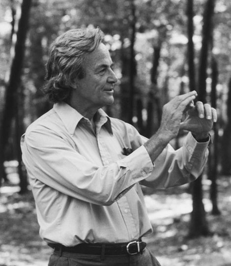
Portrait of Richard Feynman

Richard Feynman
Ref: Wikipedia

▲
Ref: https://en.wikipedia.org/wiki/Richard_Feynman


Three classical bits

There are \(2^3=8\) possible strings.

\(000,001,010,011,100,101,110,111\)

At one instant, the register contains only one of them, such as \(101\).

Memory needed: 3 bits

Three qubits

A general three-qubit state has \(2^3=8\) amplitudes:

\[ \begin{align*} \lvert\psi\rangle= &\sum_{k=0}^{7}c_k\lvert k\rangle\\ =&c;_0\lvert 000\rangle+c_1\lvert 001\rangle +c_2\lvert 010\rangle+c_3\lvert 011\rangle\\ &+c_4\lvert 100\rangle +c_5\lvert 101\rangle+c_6\lvert 110\rangle+c_7\lvert 111\rangle\\ \end{align*} \]

A simulator stores all 8 complex amplitudes, \(c_k=\alpha_k+i\beta_k\).

8-byte double precision (= 64 bits)

About 16 significant decimal digits. For example,

\(\alpha_k\approx0.1234567890123457\)
\(\beta_k\approx-0.3141592653589793\)

Real 8 B + imaginary 8 B = 16 B per amplitude.

3 qubits: \(8\times16\ \mathrm{B}=128\ \mathrm{B} \left(=1024 \mathrm{ bits} \right)\)

50-qubit state vector \(2^{50}\times16\ \mathrm{B}=16\ \mathrm{PiB}\approx18.0\ \mathrm{PB}\)

Why Shor's Algorithm Threatens RSA

RSA publishes \(N=pq\), the product of two large secret primes. Multiplying is easy; recovering \(p\) and \(q\) from \(N\) is believed to be extremely costly classically — and once you have them, the private key follows.

Shor's key step: turn factoring into period finding, which a large fault-tolerant quantum computer does in polynomial time.
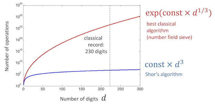
Comparison of classical number-field-sieve and Shor-algorithm operation counts as the number of digits increases
Classical factoring grows much faster than Shor's polynomial scaling · Chris Ferrie, Medium
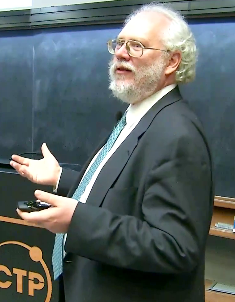
Portrait of Peter Shor
Peter Shor
Ref: Wikipedia

▲
Ref: https://en.wikipedia.org/wiki/Peter_Shor


Keys in use today

2048 bits

\(\approx617\) decimal digits. NIST wants 3072 bits beyond 2030. The classical record is RSA-250 — only 250 digits, in 2020.

Perfect qubits Shor needs

\(\sim\)4,100 logical

About \(2n+3\) for an \(n\)-bit modulus. These are idealised, error-free qubits — nobody has one.

After error correction

\(10^{6}\)–\(10^{7}\) physical

The surface code spends thousands of physical qubits per logical one: 20 million qubits / 8 hours (Gidney & Ekerå 2021), cut to under 1 million / a few days by 2025.

Prototypes today

\(10^{2}\)–\(10^{3}\) physical

IBM Heron 156, Google Willow 105, IBM Condor 1,121 — all noisy, none fault-tolerant. Roughly four orders of magnitude short.

Three Molecules Sampled on an IBM Heron QPU
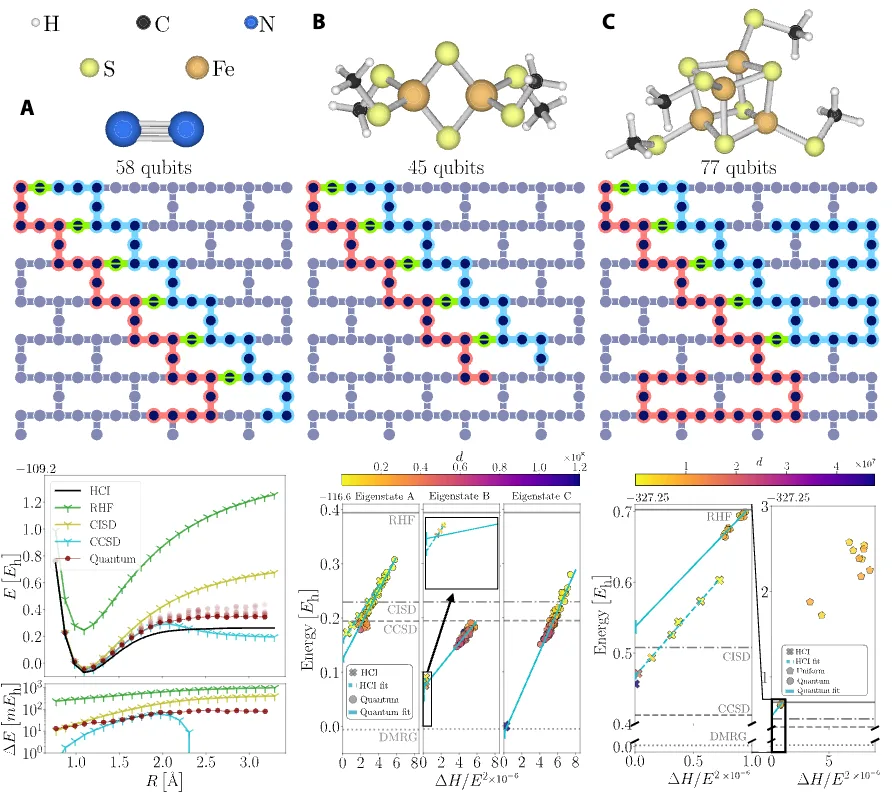
Paper figure 4: nitrogen and two iron-sulfur clusters, their Heron qubit layouts, and the resulting energy plots
Fig. 4 · Science Advances 11, eadu9991 (2025)
\(N_2\)breaking the triple bond · 58 qubits
[2Fe–2S]iron–sulfur cluster · 45 qubits
[4Fe–4S]larger cluster · 77 qubits

What they did

The Heron QPU never computes an energy. It samples electronic configurations — which orbitals are occupied. Fugaku then takes the configurations that came back, builds a small subspace out of them, and diagonalizes that classically. This is sample-based quantum diagonalization.

What came out

The \(N_2\) curve stays close to the reference right through bond breaking, where restricted CCSD falls apart. For the iron–sulfur clusters, hardware samples gave lower energies than uniformly random ones at the same subspace size — chemical signal survived a deep, noisy circuit.

Still a demonstration, not a quantum advantage. The paper claims no end-to-end speedup, and on the largest case — [4Fe–4S] at 77 qubits — leading classical methods still produced better solutions. What it shows is that a noisy QPU can be a useful sampler inside a classical workflow.

Syllabus
𝒊𝑁𝑆𝐼𝐺𝐻𝑇 𝒊ℏ
PHYS598500 · Week 1 Computation Is Physical · Manual Slides
Slide previews—
01/ —