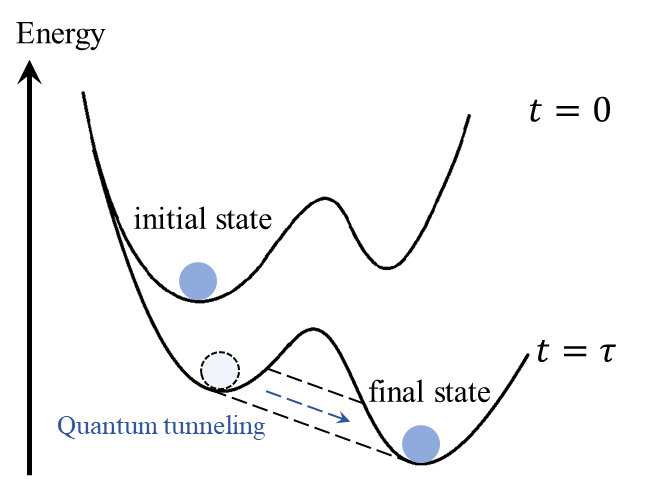
PHYS598500 · Week 1 · T1
Computation Is Physical
From Mechanized Reasoning to Quantum Hardware and the Limits of Physics
Why Must Computer Science Eventually Meet Physics?
→Because computation needs hardware.
In physics, we study:
Matter
the hardware itself
Energy–momentum transfer
how we control the hardware
State evolution
how the algorithm is encoded
Click the slide or press → to reveal one layer; press ← to hide it again.
Q1. Can Calculation and Reasoning Be Mechanized?
From Human Procedure to Symbolic State Transformation
Charles Babbage: From Automatic Tables to a Programmable Machine
Charles Babbage (1791–1871) first designed the Difference Engine to automate numerical tables. Finite differences reduce polynomial tabulation to repeated addition, making the task suitable for a gear-based mechanism and reducing human calculation and typesetting errors.
The later Analytical Engine was a general architecture. It separated a “store” from a “mill,” used punched cards to specify operations and data, and included sequencing, repetition, and conditional control.
| Design | Modern analogy |
|---|---|
| Store | Memory |
| Mill | Arithmetic/processing unit |
| Punched cards | Program and data input |
| Operation sequence | Control flow |
Caution: the full Analytical Engine was not completed in Babbage's lifetime.
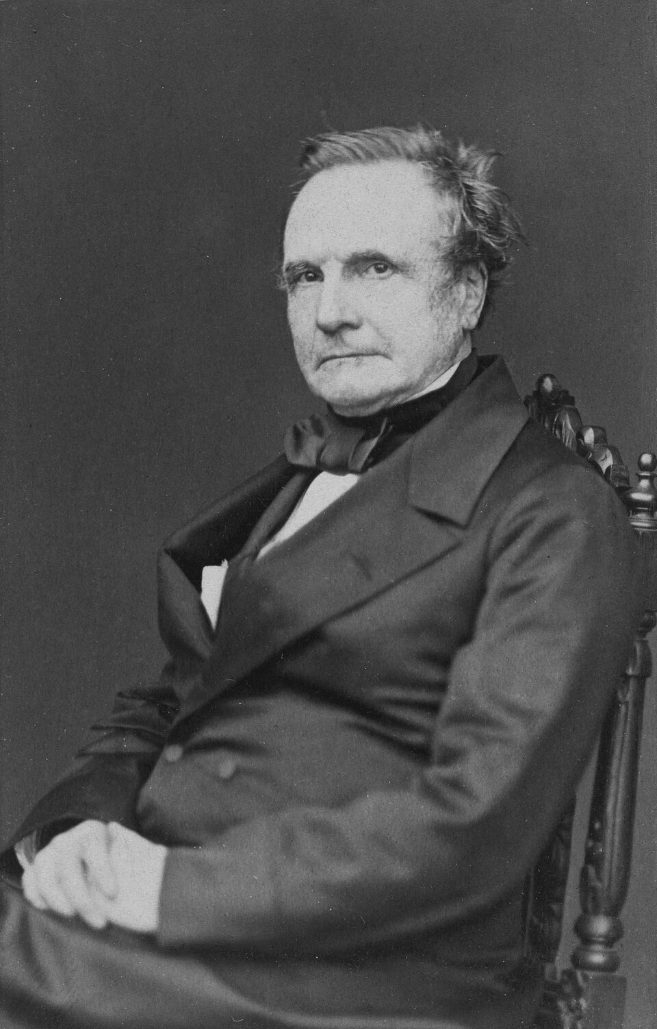
Why Mechanize Tables? Checking Still Failed
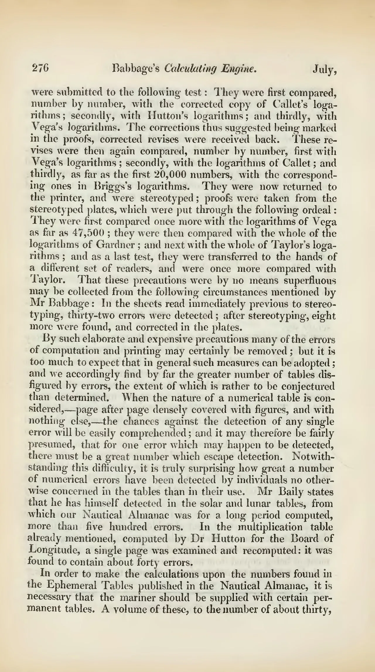
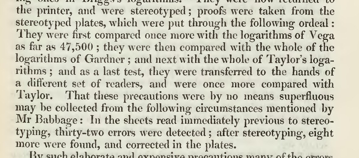
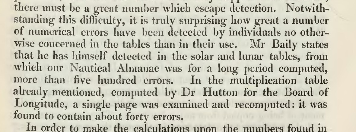
Same Page, Two Copied Errors: Hutton vs. Babbage
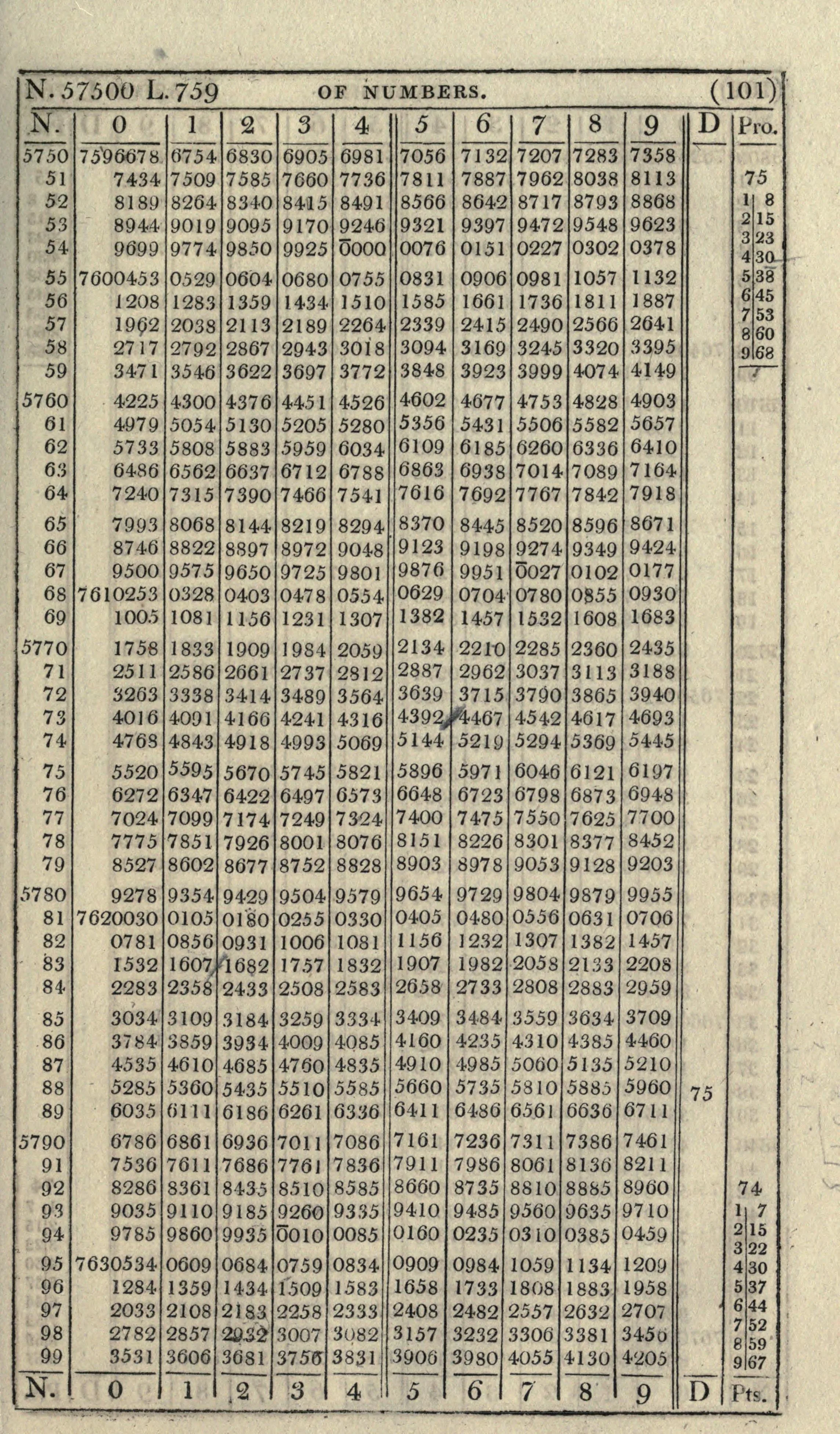
 wrong
wrong
57,628 → …633657,629 → …6410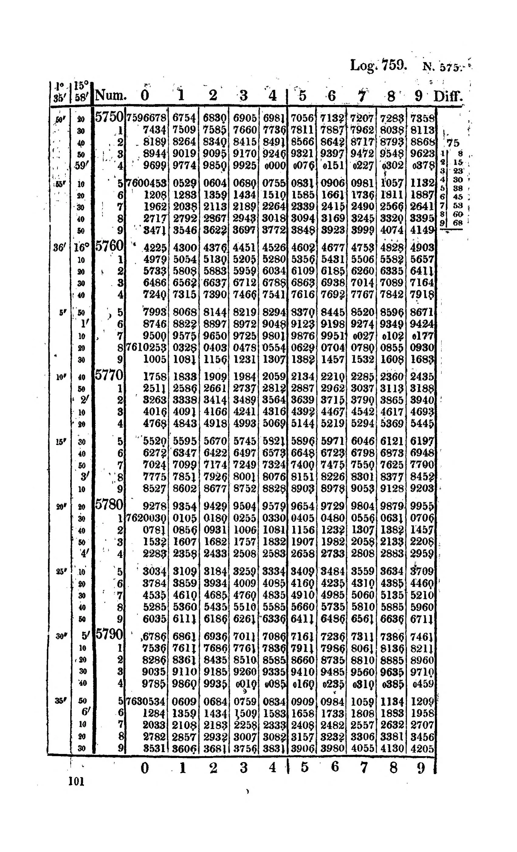
 correct
57,628 → …633557,629 → …6411Seven-place common (base-10) logarithms: the page prints only the last four mantissa digits, the leading \(760\) coming from the block header N. 57500 L. 759.
\(\log_{10}57628=4.7606335\)Hutton …6336
\(\log_{10}57629=4.7606411\)Hutton …6410
Difference Engine No. 2: Built in Metal
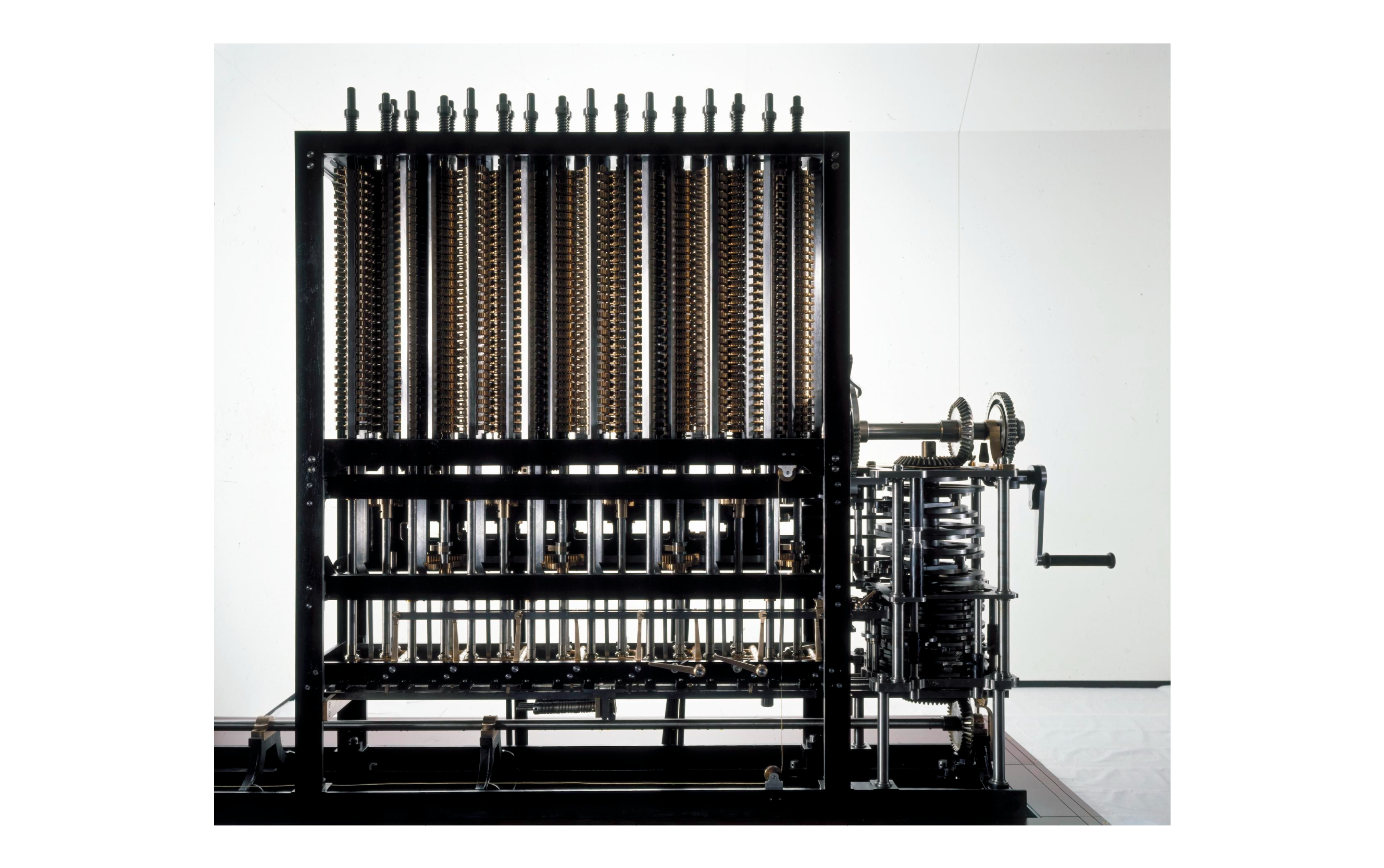
Complete
reconstruction
Ref:
Science Museum Group Collection
▲
Ref:
https://collection.sciencemuseumgroup.org.uk/objects/co62748/babbages-difference-engine-no-2-2002
拷貝.png)
Decimal figure wheels and gear
trains
Ref:
Science Museum Group Collection
▲
Ref:
https://collection.sciencemuseumgroup.org.uk/objects/co62748/babbages-difference-engine-no-2-2002
Difference Engine No. 2: From Drawings to Mechanism
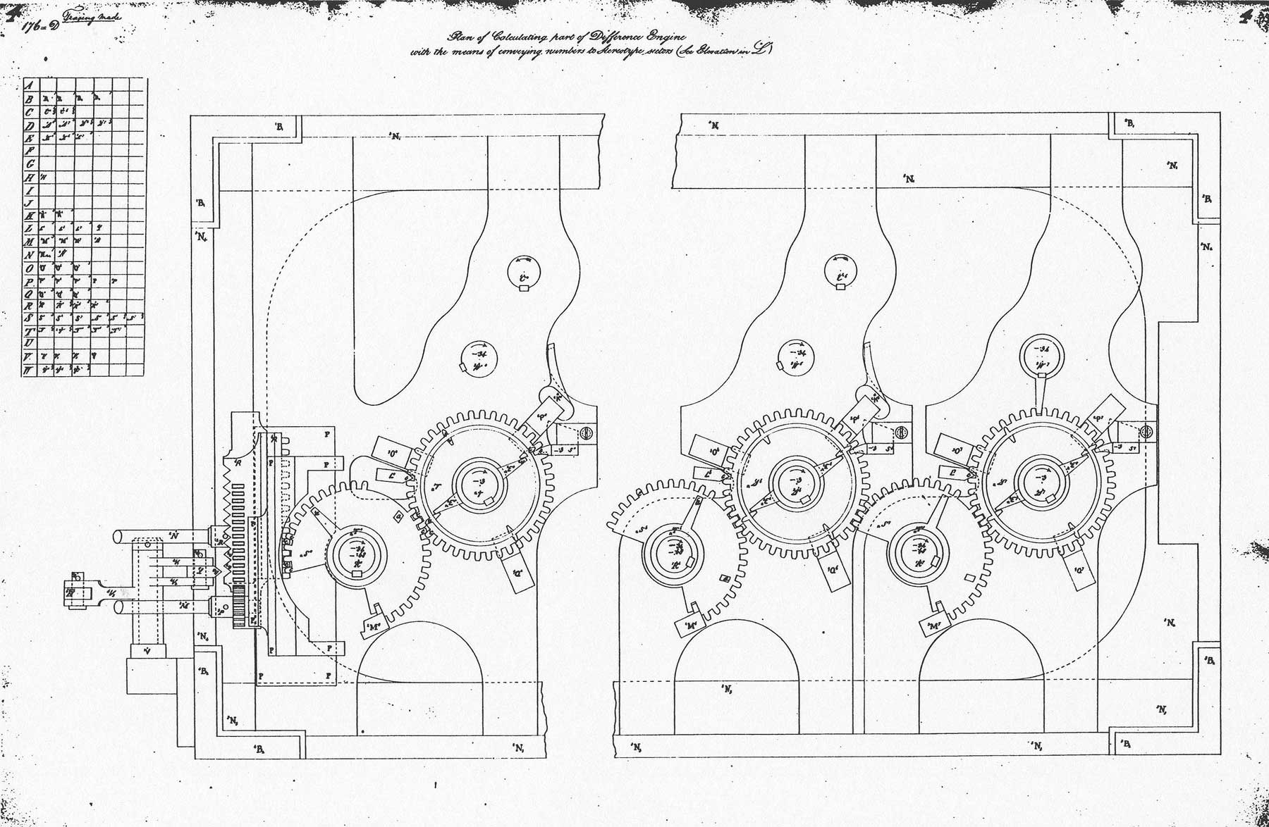
Plan of the calculating
mechanism
Ref:
Cronatec · How did the Difference Engine work?
▲
Ref:
https://cronatec.ch/how-did-the-difference-engine-work/
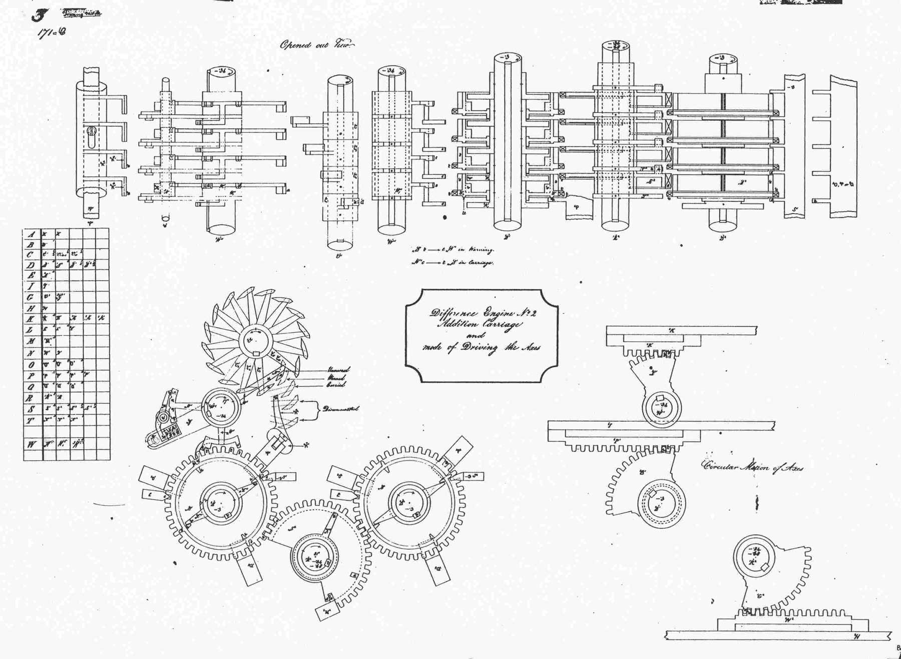
Addition and carriage
mechanisms
Ref:
Cronatec · How did the Difference Engine work?
▲
Ref:
https://cronatec.ch/how-did-the-difference-engine-work/
Analytical Engine: Mechanism and Punched-Card Control

Ref: Science Museum Group Collection
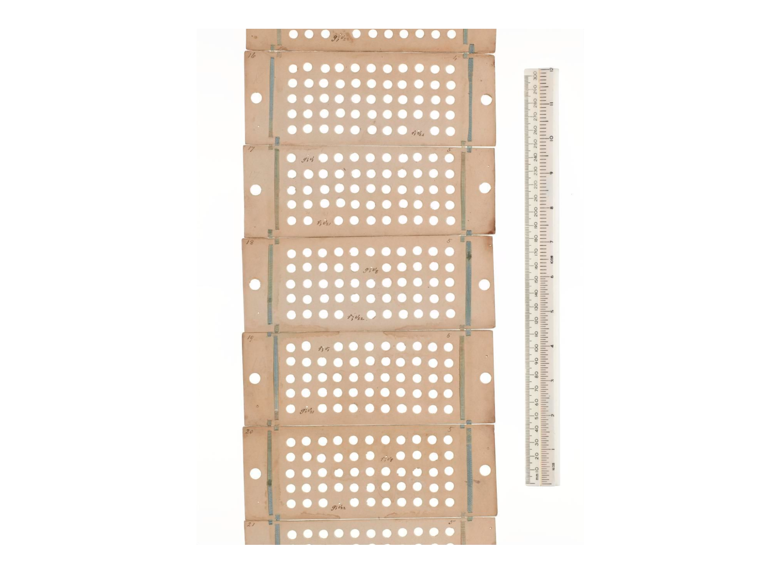
Ref: Science Museum Group Collection
Why the Analytical Engine Was a Conceptual Breakthrough
The Difference Engine mechanized a specialized mathematical task. The Analytical Engine asked a deeper question: can the same machine perform many tasks when its sequence of operations is changed?
\[\boxed{\text{fixed-purpose mechanism}\rightarrow\text{programmable general-purpose architecture}.}\]
This anticipates three distinctions that remain essential:
- Machine: the physical system and its available elementary operations.
- Program: an encoded sequence that selects and organizes those operations.
- Data: the encoded objects on which the operations act.
Babbage did not build a functioning modern computer, and the Analytical Engine was not a Turing machine formulated a century early. Its importance is architectural: it made programmable, automatic symbolic procedure imaginable as a machine design.
Boole: Logic Becomes Algebra
Boole showed that logical statements can be represented by symbols and manipulated with algebraic rules.
For Boolean variables \(a,b\in\{0,1\}\), logical AND behaves exactly like multiplication:
Logic: \(a\ \mathrm{AND}\ b\)
| \(a\) | \(b\) | \(a\land b\) |
|---|---|---|
| 0 | 0 | 0 |
| 0 | 1 | 0 |
| 1 | 0 | 0 |
| 1 | 1 | 1 |
Algebra: \(a*b\)
| \(a\) | \(b\) | \(a*b\) |
|---|---|---|
| 0 | 0 | 0 |
| 0 | 1 | 0 |
| 1 | 0 | 0 |
| 1 | 1 | 1 |
For \(a,b\in\{0,1\}\), \(a\land b=a*b\).
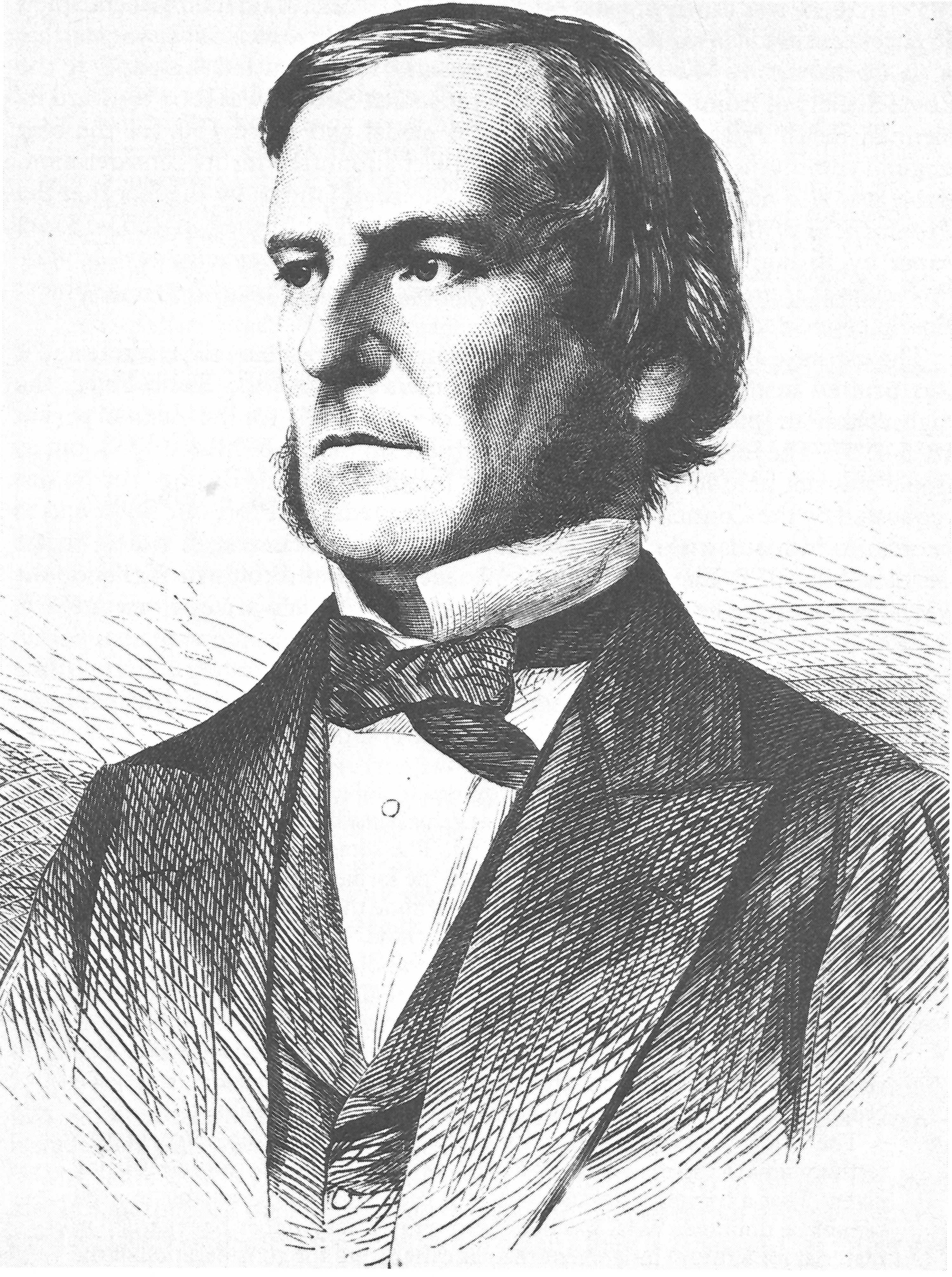
George Boole
Ref:
Wikipedia
Shannon: Boolean Algebra Becomes Switching-Circuit Design
Claude Shannon (1916–2001) showed that the ON/OFF behavior of relay circuits follows Boolean algebra. A switch is OFF when the circuit is open and ON when a conducting path is closed. We encode OFF as \(0\) and ON as \(1\).
| Connection | Boolean operation |
|---|---|
| Series: output is ON only when \(a\) and \(b\) are ON | \(a\land b\) |
| Parallel: output is ON when \(a\) or \(b\) is ON | \(a\lor b\) |
| Normally closed: output is ON when \(a\) is OFF | \(\neg a\) |
\[\boxed{\text{Boolean expression}\longleftrightarrow\text{switching network}.}\]
This made circuit design systematic: specify the desired ON/OFF output, express and simplify it with Boolean algebra, then connect switches that realize the same relation.
.jpg)
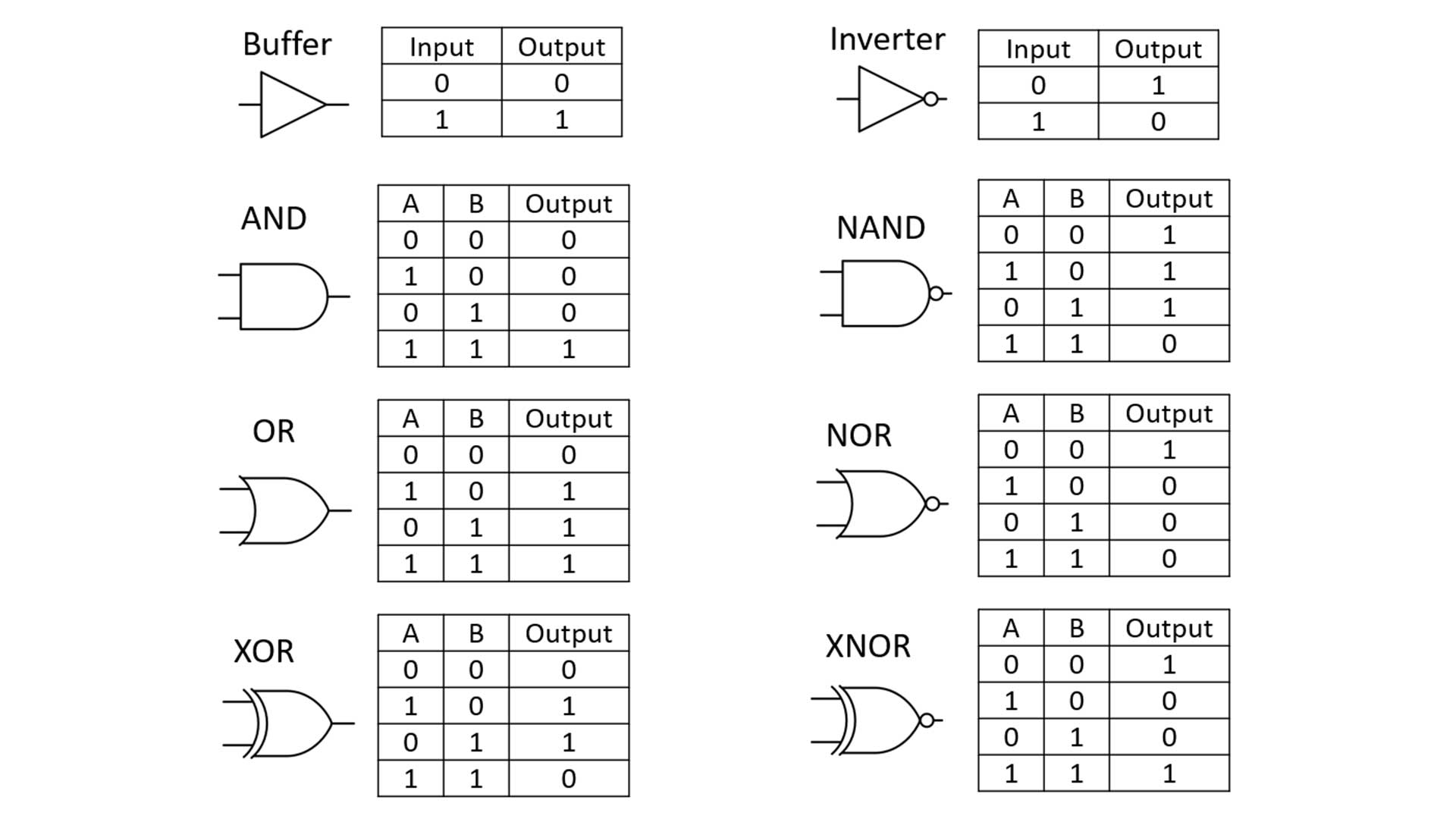
Logic Gates Implement Boolean Functions
Let \(A=\{a=1\}\) and \(B=\{b=1\}\). The shaded region is where the output equals \(1\).
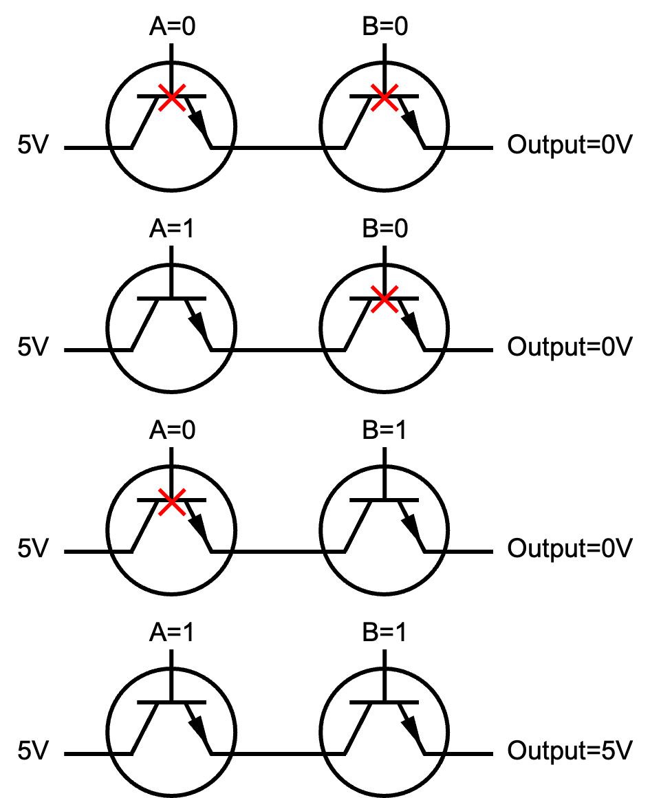
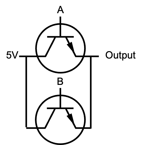
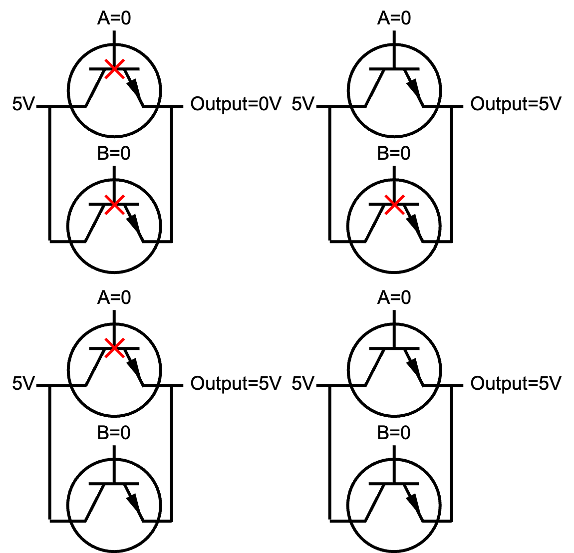
A physical switch, relay, or transistor realizes the same Boolean relation.
\[\mathrm{NOT}:a\mapsto\neg a\]
\[\mathrm{AND}:(a,b)\mapsto a\land b\]
Gates become useful when their outputs are composed into a larger circuit.
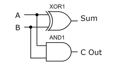
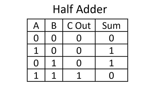
Half adder: AND → Carry; XOR → Sum
Universal Gate Set
A universal gate set can express every Boolean function.
- \(\{\mathrm{AND},\mathrm{NOT}\}\) is universal.
- \(\{\mathrm{OR},\mathrm{NOT}\}\) is universal.
- \(\{\mathrm{NAND}\}\) alone is universal.
- \(\{\mathrm{NOR}\}\) alone is universal.
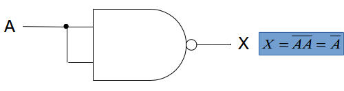

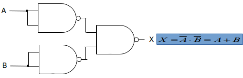
Because NAND reproduces NOT, AND, and OR, NAND alone can generate every Boolean circuit.
Figures: CUNY OpenLab, Lab 05 · CC BY-NC-SA 3.0 · resized.
Q2. How we encode algorithm into physical evolution?
From Reversible Boolean Functions to Unitary and Hamiltonian Evolution
Semiconductor Fabrication
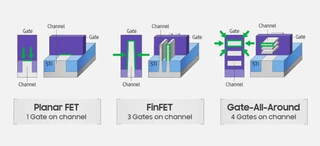
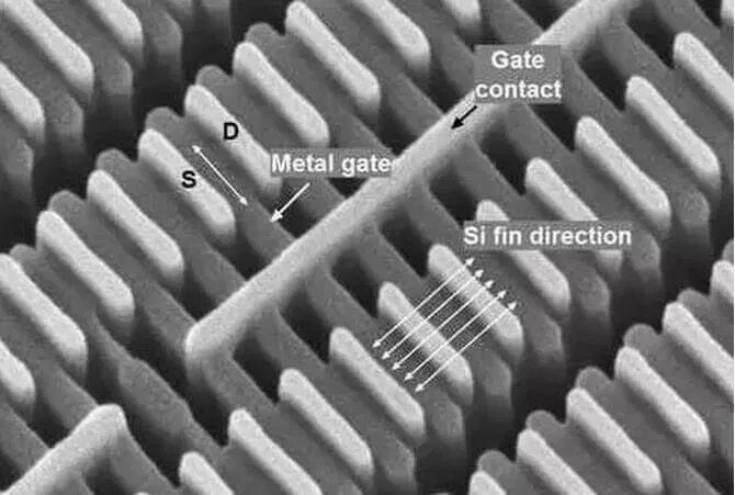
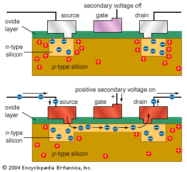
Refs: Britannica · UTMEL · Deep Forest
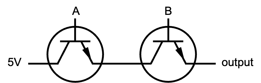
AND Gate:Series Switches
OR Gate:Parallel Switches
Flash Memory
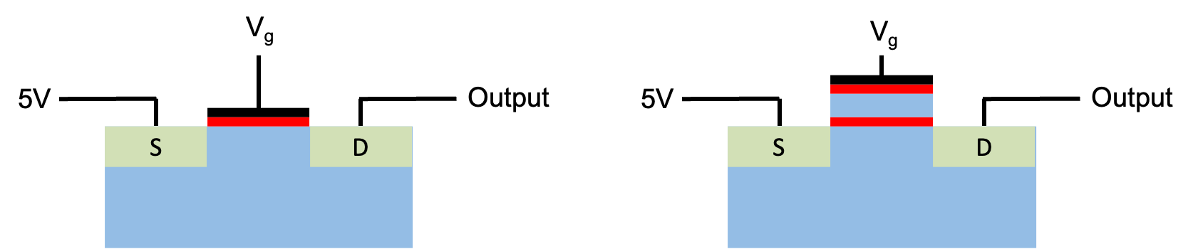
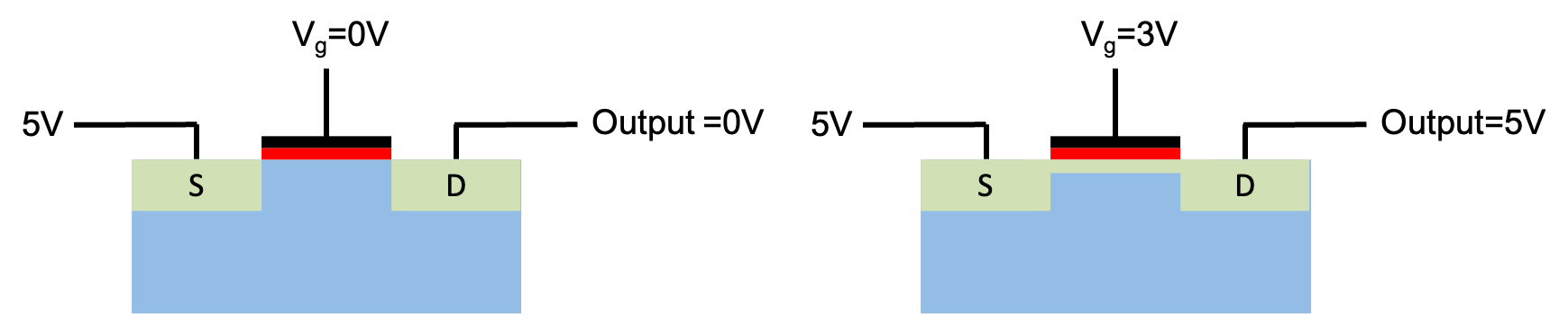
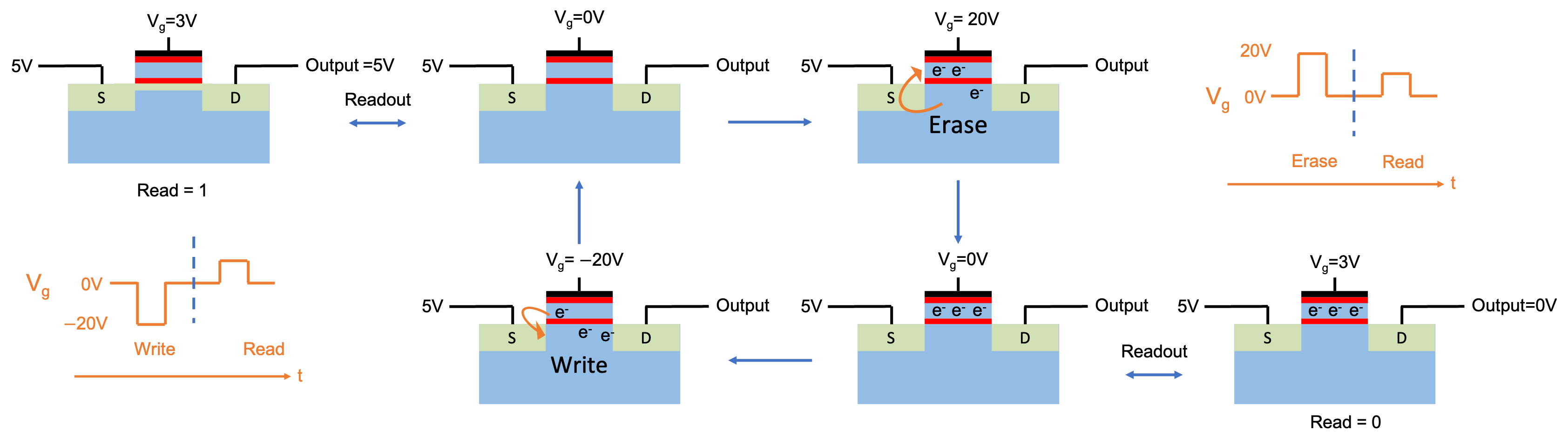
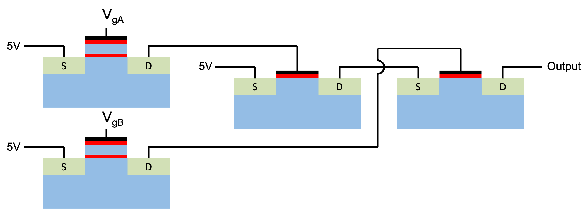
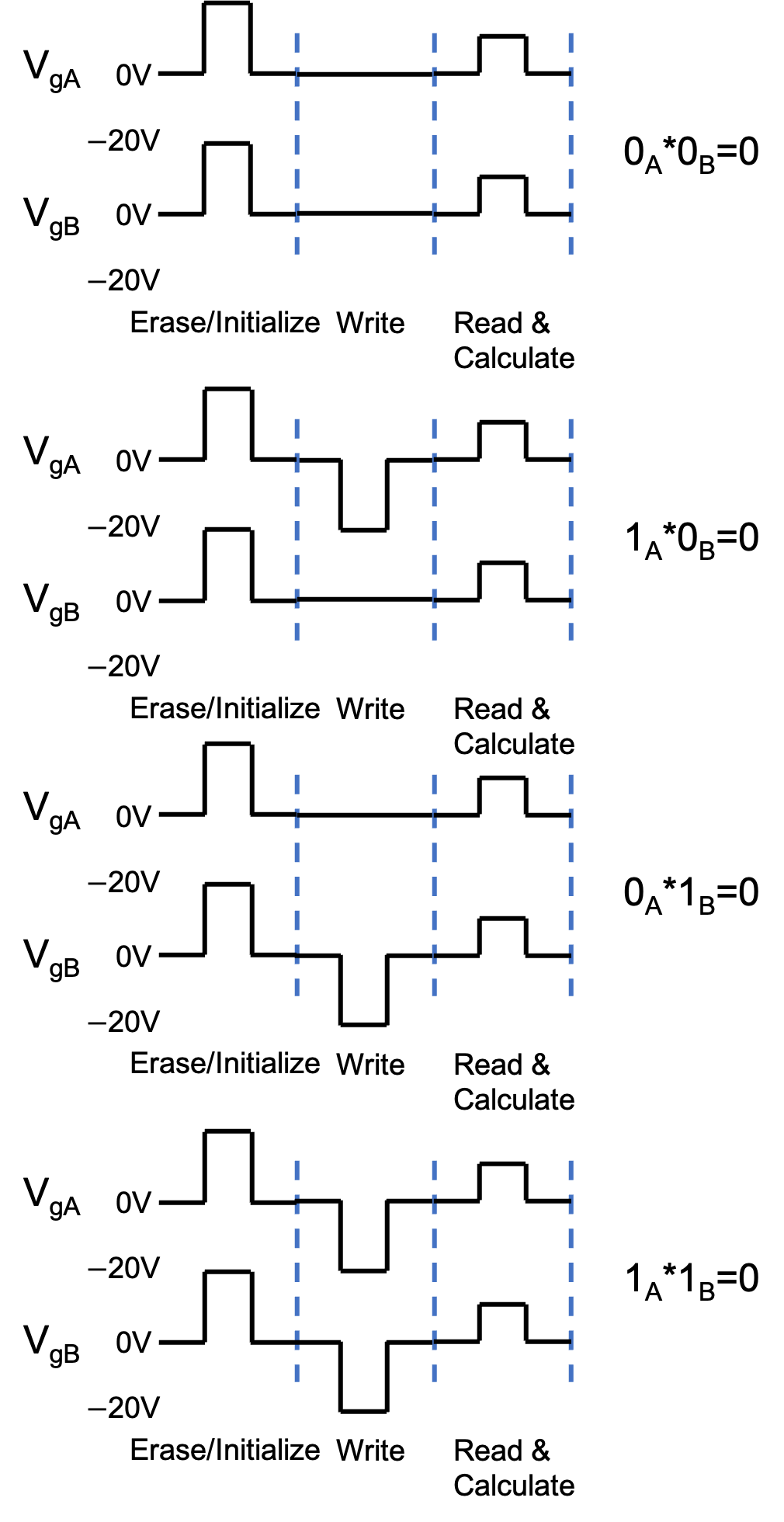
An algorithm or program is mapped onto a timed control waveform \(V(t)\).
\(H(t)=H_{\mathrm{hardware}}+V(t)\)
A quantum algorithm or program is realized as controlled evolution under a time‑dependent Hamiltonian \(H(t)\).
From Reversible Logic to Physical Evolution
\[i\hbar\frac{d}{dt}|\psi(t)\rangle=H(t)|\psi(t)\rangle,\]
\[U(T,0)=\mathcal T\exp\!\left[-\frac{i}{\hbar}\int_0^T H(t)\,dt\right],\]
\[|\psi(T)\rangle=U(T,0)|\psi(0)\rangle.\]
\[\boxed{\text{Reversibility}:\exists U^{-1} \text{ s.t } U*U^{-1}=I}\]
\[U^{-1}(T,0)=U(0,T)=U^\dagger(T,0)=\mathcal T\exp\!\left[\textcolor{red}{+}\frac{i}{\hbar}\int_0^T H(t)\,dt\right]\]
\[\langle \psi(T)|\psi(T)\rangle=\langle \psi(0)|U^\dagger(T,0)* U(T,0)|\psi(T)\rangle=\langle \psi(0)|\psi(0)\rangle=1\]
\[\begin{align*}
U(T,0)&\approx \mathcal T\exp\!\left[-\frac{i}{\hbar}\int_{T_n}^T H(t)\,dt\right]*\mathcal
T\exp\!\left[-\frac{i}{\hbar}\int_{T_{n-1}}^{T_n} H(t)\,dt\right]*...*\mathcal
T\exp\!\left[-\frac{i}{\hbar}\int_0^{T_1} H(t)\,dt\right],\\
&\approx U(T,T_n)*U(T_n,T_{n-1})*...*U(T_1,0)
\end{align*}\]
\[\boxed{\text{Boolean function}\rightarrow\text{reversible embedding}\rightarrow\text{unitary}\rightarrow H(t).}\]
Information Erasure Makes Logic Irreversible
A gate is reversible only when its output identifies one unique input.
Erasing one unbiased bit requires the environment to receive at least
\[\Delta S_{\mathrm{env}}\ge k_B\ln2\]
\[Q_{\min}\ge k_BT\ln2\]
Half adder: \(01\) and \(10\) both produce \((\mathrm{Carry},\mathrm{Sum})=(0,1)\).
Source: Landauer (1961).
Controlled Gates Preserve Their Inputs
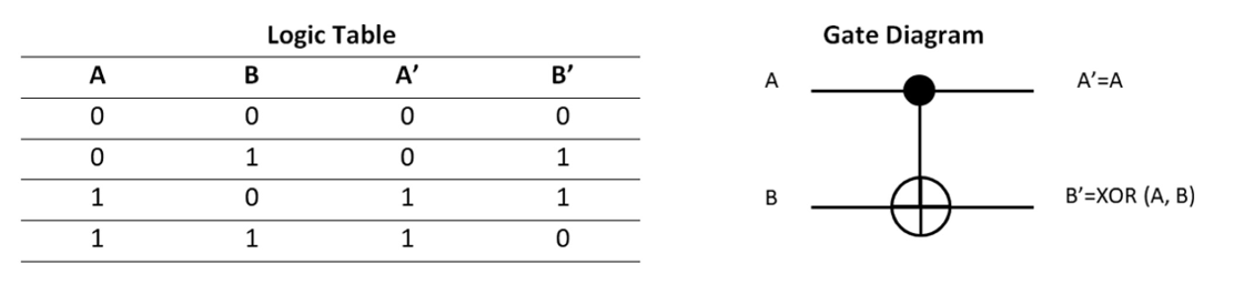
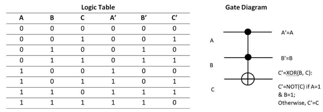
A Reversible Half Adder Keeps Enough Information
Conventional: information is lost
| A | B | Carry | Sum |
|---|---|---|---|
| 0 | 0 | 0 | 0 |
| 0 | 1 | 0 | 1 |
| 1 | 0 | 0 | 1 |
| 1 | 1 | 1 | 0 |
01 and 10 both give (Carry, Sum) = (0, 1).
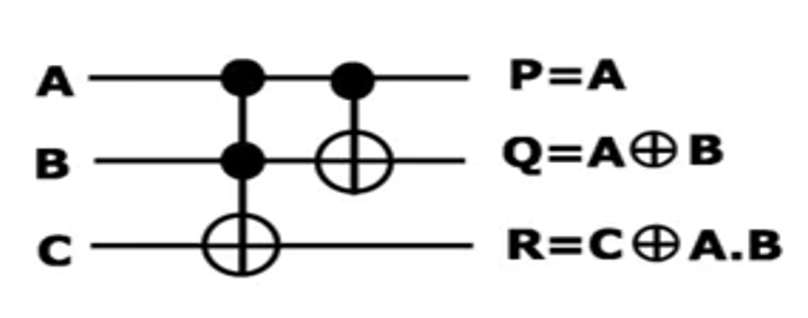
Reversible embedding: retain one input
| A | B | C | P | R = Carry | Q = Sum |
|---|---|---|---|---|---|
| 0 | 0 | 0 | 0 | 0 | 0 |
| 0 | 1 | 0 | 0 | 0 | 1 |
| 1 | 0 | 0 | 1 | 0 | 1 |
| 1 | 1 | 0 | 1 | 1 | 0 |
With C = 0, P = A preserves the input, so 01 and 10 remain distinct.
Q3. How we encode algorithm into QUANTUM physical evolution?
From Reversible Logic to Physical Evolution
\[i\hbar\frac{d}{dt}|\psi(t)\rangle=H(t)|\psi(t)\rangle,\]
\[U(T,0)=\mathcal T\exp\!\left[-\frac{i}{\hbar}\int_0^T H(t)\,dt\right],\]
\[|\psi(T)\rangle=U(T,0)|\psi(0)\rangle.\]
\[\boxed{\text{Reversibility}:\exists U^{-1} \text{ s.t } U*U^{-1}=I}\]
\[U^{-1}(T,0)=U(0,T)=U^\dagger(T,0)=\mathcal T\exp\!\left[\textcolor{red}{+}\frac{i}{\hbar}\int_0^T H(t)\,dt\right]\]
\[\langle \psi(T)|\psi(T)\rangle=\langle \psi(0)|U^\dagger(T,0)* U(T,0)|\psi(T)\rangle=\langle \psi(0)|\psi(0)\rangle=1\]
\[\begin{align*}
U(T,0)&\approx \mathcal T\exp\!\left[-\frac{i}{\hbar}\int_{T_n}^T H(t)\,dt\right]*\mathcal
T\exp\!\left[-\frac{i}{\hbar}\int_{T_{n-1}}^{T_n} H(t)\,dt\right]*...*\mathcal
T\exp\!\left[-\frac{i}{\hbar}\int_0^{T_1} H(t)\,dt\right],\\
&\approx U(T,T_n)*U(T_n,T_{n-1})*...*U(T_1,0)
\end{align*}\]
\[\boxed{\text{Boolean function}\rightarrow\text{reversible embedding}\rightarrow\text{unitary}\rightarrow H(t).}\]
Visualizing a Qubit State on the Bloch Sphere
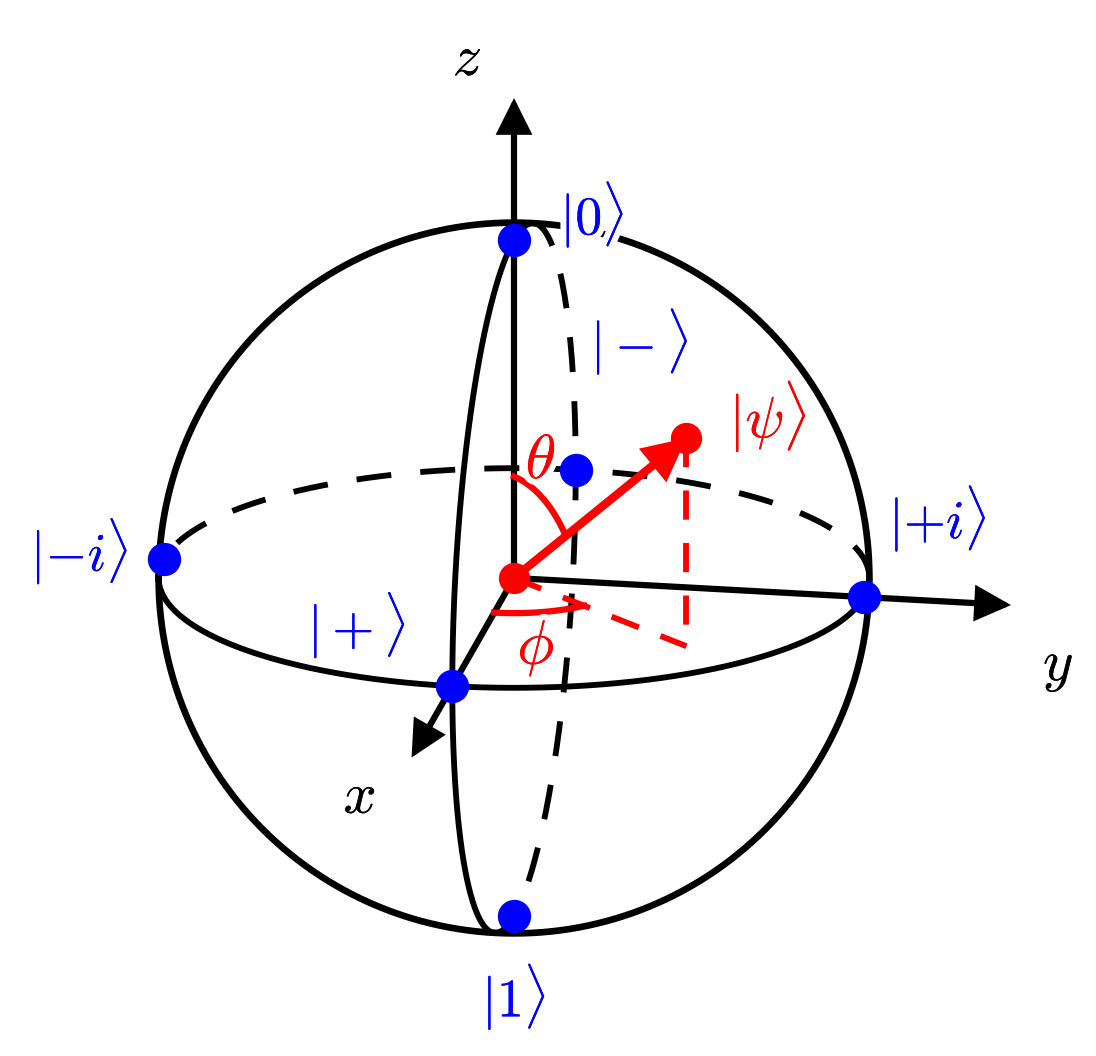
For any two state system with orthonormal basis \(|a \rangle, \ |b \rangle\) \[|\psi\rangle = c_0 |a \rangle + c_1 |b \rangle,\quad c_k=|c_k|e^{i\phi_k}\in \mathbb{C},\quad \langle a|b \rangle=0\] \[\left\{ \begin{array}{c} \langle \psi|\psi \rangle=1 \to |c_0|^2+|c_1|^2=1 \\ \text{unobservable global phase }\phi_0 \end{array} \right.\] \[|\psi(\theta,\phi)\rangle =\cos\!\left(\frac{\theta}{2}\right)|a\rangle +e^{i\phi}\sin\!\left(\frac{\theta}{2}\right)|b\rangle \]
\(0\leq\theta\leq\pi,\qquad 0\leq\phi< 2\pi\)
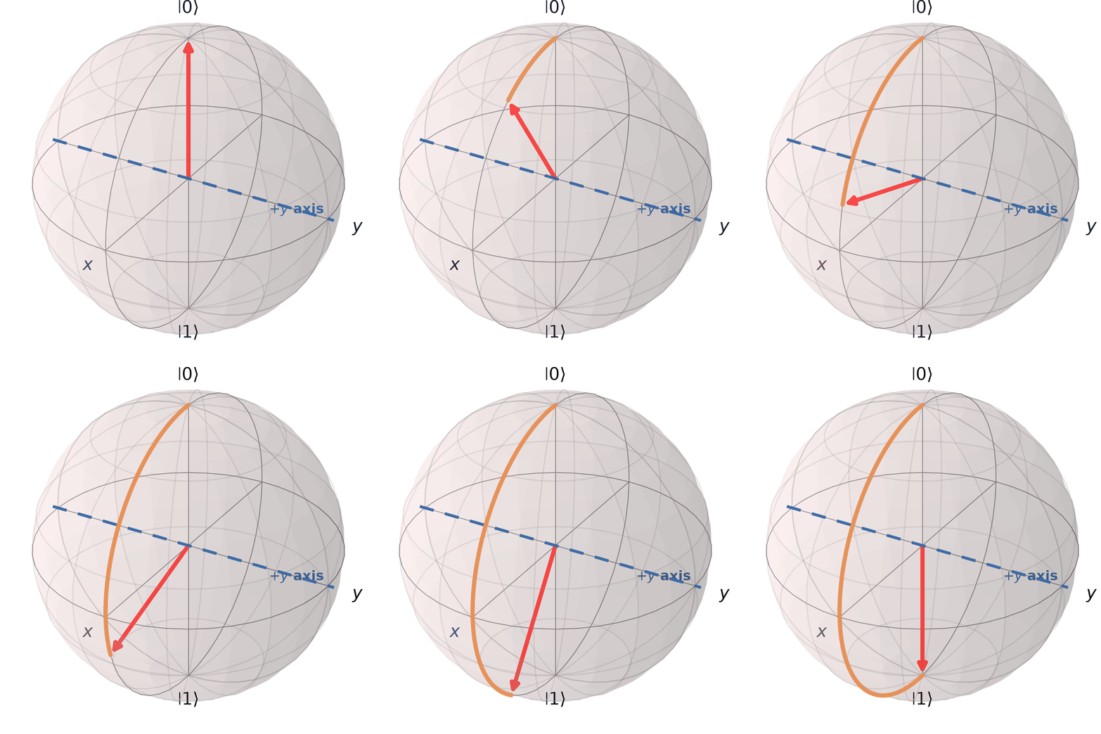
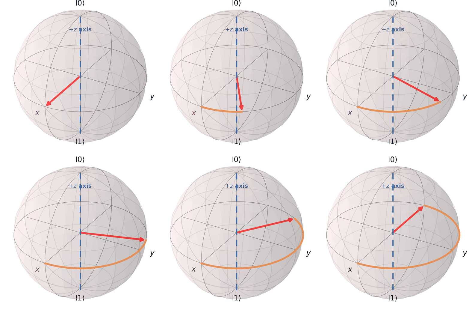
Pauli-\(Z\) gate and Z-axis
\(\left\{
\begin{array}{c}
Z|0\rangle=+|0\rangle \\
Z|1\rangle=-|1\rangle
\end{array}
\right.\)
Pauli-\(X\) gate and X-axis
\(\left\{
\begin{array}{c}
X|+\rangle=+|+\rangle \\
X|-\rangle=-|-\rangle
\end{array}
\right.\)
Pauli-\(Y\) gate and Y-axis
\(\left\{
\begin{array}{c}
Y|i\rangle=+|i\rangle \\
Y|-i\rangle=-|-i\rangle
\end{array}
\right.\)
We normally choose \(|0 \rangle, \ |1 \rangle\) as our orthonormal basis \(|0 \rangle=\left( \begin{array}{c} 1 \\ 0 \end{array} \right), \ |1 \rangle =\left( \begin{array}{c} 0 \\ 1 \end{array} \right), \ |\psi \rangle =\left( \begin{array}{c} \cos\!\left(\frac{\theta}{2}\right) \\ e^{i\phi}\sin\!\left(\frac{\theta}{2}\right) \end{array} \right) \)
\[|\psi\rangle = c_0 |0 \rangle + c_1 |1 \rangle, c_k=|c_k|e^{i\phi_k}\in \mathbb{C}\]
\[|c_0|^2+|c_1|^2=1 \to
\left\{
\begin{array}{c}
|c_0|\equiv \cos \left( \frac{\theta}{2} \right) \\
|c_1|\equiv \sin \left( \frac{\theta}{2} \right)
\end{array}
\right.\]
\[\begin{align*} |\psi\rangle &= \cos \left( \frac{\theta}{2} \right) \ e^{i\phi_0} |0 \rangle + \sin \left( \frac{\theta}{2} \right) \ e^{i\phi_1} |1 \rangle\\ &=e^{i\phi_0}\left[ \cos \left( \frac{\theta}{2} \right) \ |0 \rangle + \sin \left( \frac{\theta}{2} \right) \ e^{i\left(\phi_1-\phi_0\right)} |1 \rangle \right]\\ &\equiv e^{i\phi_0}\left[ \cos \left( \frac{\theta}{2} \right) \ |0 \rangle + \sin \left( \frac{\theta}{2} \right) \ e^{i\phi} |1 \rangle \right] \qquad =e^{i \phi_0 } \left( \begin{array}{c} \cos \left( \frac{\theta}{2} \right) \\ e^{i\phi}\sin \left( \frac{\theta}{2} \right) \end{array} \right) \end{align*}\]
Density matrix \(\rho\):
\[\begin{align*}
\rho &\equiv |\psi \rangle \langle \psi |
=e^{i\phi_0}
\begin{pmatrix}
\cos\left( \frac{\theta}{2} \right) \\
e^{i\phi}\sin\left( \frac{\theta}{2} \right)
\end{pmatrix}
\otimes
e^{-i\phi_0}
\begin{pmatrix}
\cos\left( \frac{\theta}{2} \right) & e^{-i\phi}\sin\left( \frac{\theta}{2} \right)
\end{pmatrix} \\
&=
\begin{pmatrix}
\cos^2\left( \frac{\theta}{2} \right)
&
e^{-i\phi}\sin\left( \frac{\theta}{2} \right)\cos\left( \frac{\theta}{2} \right)
\\
e^{i\phi}\sin\left( \frac{\theta}{2} \right)\cos\left( \frac{\theta}{2} \right)
&
\sin^2\left( \frac{\theta}{2} \right)
\end{pmatrix}
\\
&=
\frac{1}{2}\begin{pmatrix}
1+\cos \theta
&
e^{-i\phi}\sin \theta
\\
e^{i\phi}\sin \theta
&
1-\cos \theta
\end{pmatrix}
\end{align*}\]
\[|\psi\rangle = \cos \left( \frac{\theta}{2} \right) \ |0 \rangle + \sin \left( \frac{\theta}{2} \right) \ e^{i\phi} |1 \rangle \]
\[|\psi\rangle = e^{i\phi_0}\left[ \cos \left( \frac{\theta}{2} \right) \ |0 \rangle + \sin \left( \frac{\theta}{2} \right) \ e^{i\phi} |1 \rangle \right] \]
Density matrix \(\rho\):
\[\begin{align*}
\rho &\equiv |\psi \rangle \langle \psi |
=
\frac{1}{2}\begin{pmatrix}
1+\cos \theta
&
e^{-i\phi}\sin \theta
\\
e^{i\phi}\sin \theta
&
1-\cos \theta
\end{pmatrix}\\
\\
&=
\frac{1}{2}\begin{pmatrix}
1+\cos \theta
&
\cos \phi \sin \theta - i\sin \phi \sin \theta
\\
\cos \phi \sin \theta + i\sin \phi \sin \theta
&
1-\cos \theta
\end{pmatrix}\\
\\
&=
\frac{1}{2}\left[
\begin{pmatrix}
1&0\\
0&1
\end{pmatrix}
+ \cos \phi \sin \theta \begin{pmatrix}
0&1\\
1&0
\end{pmatrix}
+\sin \phi \sin \theta \begin{pmatrix}
0&-i\\
i&0
\end{pmatrix}
+\cos \theta \begin{pmatrix}
1&0\\
0&-1
\end{pmatrix}
\right]\\
&\equiv
\frac{1}{2}\left[
I
+ r_x \sigma_x
+ r_y \sigma_y
+ r_z \sigma_z
\right]
\end{align*}\]
Single-Qubit Rotation Operators
\[ \begin{align*} H&= cI + h_x\sigma_x +h_y\sigma_y +h_z\sigma_z \end{align*} \]
\[ U(t)=e^{-itH}=e^{-it(cI +h_x\sigma_x +h_y\sigma_y +h_z\sigma_z)} \]
\(R_x(\alpha)\equiv e^{\left(-i\frac{\alpha}{2}\sigma_x\right)}\)
\(R_y(\alpha)\equiv e^{\left(-i\frac{\alpha}{2}\sigma_y\right)}\)
\(R_z(\alpha)\equiv e^{\left(-i\frac{\alpha}{2}\sigma_z\right)}\)
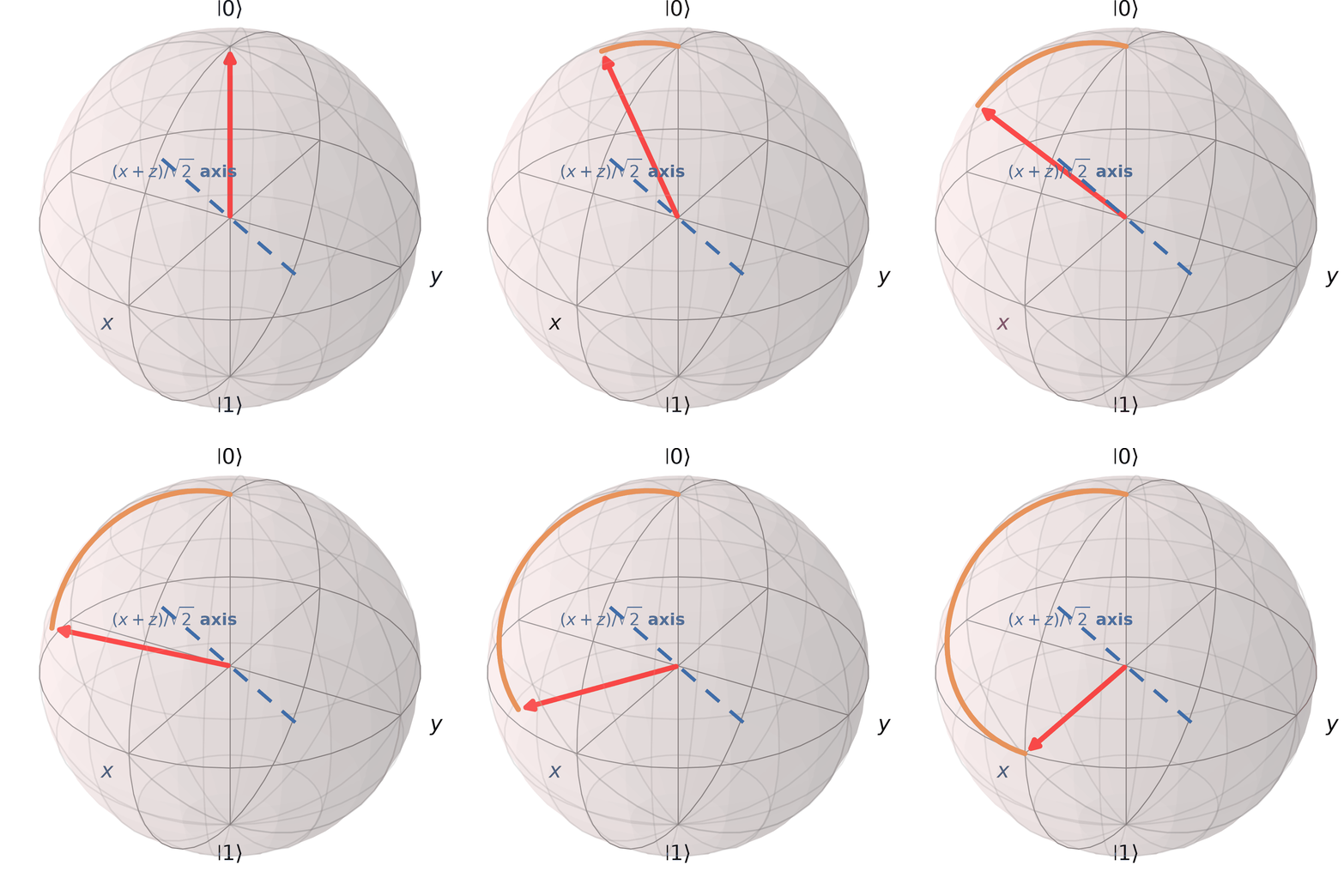
\(R_{\hat{\mathbf n}_H}(\alpha)\)
\(\hat{\mathbf n}_H=(\hat{\mathbf x}+\hat{\mathbf z})/\sqrt2\)
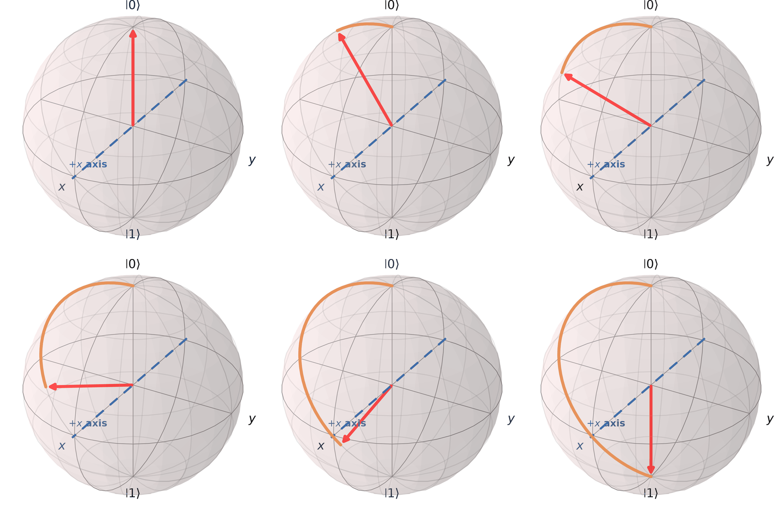
Deriving the \(x\)-Axis Bloch Rotation
\[ \rho=\frac12\left(I+r_x\sigma_x+r_y\sigma_y+r_z\sigma_z\right), \qquad U_x(\alpha)=\cos\tfrac\alpha2\,I-i\sin\tfrac\alpha2\,\sigma_x. \]
\[ U_x^\dagger\sigma_xU_x=\sigma_x. \]
\[ \begin{aligned} U_x^\dagger\sigma_yU_x &=\left(\cos\tfrac\alpha2\,I+i\sin\tfrac\alpha2\,\sigma_x\right) \sigma_y \left(\cos\tfrac\alpha2\,I-i\sin\tfrac\alpha2\,\sigma_x\right)\\ &=\cos^2\tfrac\alpha2\,\sigma_y -i\cos\tfrac\alpha2\sin\tfrac\alpha2\,\sigma_y\sigma_x +i\cos\tfrac\alpha2\sin\tfrac\alpha2\,\sigma_x\sigma_y +\sin^2\tfrac\alpha2\,\sigma_x\sigma_y\sigma_x\\ &=\left(\cos^2\tfrac\alpha2-\sin^2\tfrac\alpha2\right)\sigma_y -2\cos\tfrac\alpha2\sin\tfrac\alpha2\,\sigma_z\\ &=\cos\alpha\,\sigma_y-\sin\alpha\,\sigma_z. \end{aligned} \]
\[ \begin{aligned} U_x^\dagger\sigma_zU_x &=\left(\cos\tfrac\alpha2\,I+i\sin\tfrac\alpha2\,\sigma_x\right) \sigma_z \left(\cos\tfrac\alpha2\,I-i\sin\tfrac\alpha2\,\sigma_x\right)\\ &=\cos^2\tfrac\alpha2\,\sigma_z -i\cos\tfrac\alpha2\sin\tfrac\alpha2\,\sigma_z\sigma_x +i\cos\tfrac\alpha2\sin\tfrac\alpha2\,\sigma_x\sigma_z +\sin^2\tfrac\alpha2\,\sigma_x\sigma_z\sigma_x\\ &=2\cos\tfrac\alpha2\sin\tfrac\alpha2\,\sigma_y +\left(\cos^2\tfrac\alpha2-\sin^2\tfrac\alpha2\right)\sigma_z\\ &=\sin\alpha\,\sigma_y+\cos\alpha\,\sigma_z. \end{aligned} \]
Read off the new Bloch coordinates
\[ \rho'=U_x\rho U_x^\dagger, \qquad r_i'=\operatorname{Tr}\!\left(\rho\,U_x^\dagger\sigma_iU_x\right). \]
\[ \begin{aligned} r_x'&=r_x,\\ r_y'&=r_y\cos\alpha-r_z\sin\alpha,\\ r_z'&=r_y\sin\alpha+r_z\cos\alpha. \end{aligned} \]
\[ \begin{pmatrix}r_x'\\r_y'\\r_z'\end{pmatrix} = \begin{pmatrix} 1&0&0\\ 0&\cos\alpha&-\sin\alpha\\ 0&\sin\alpha&\cos\alpha \end{pmatrix} \begin{pmatrix}r_x\\r_y\\r_z\end{pmatrix}. \]
\[ \alpha=\frac\pi2: \qquad |0\rangle\longmapsto\frac{|0\rangle-i|1\rangle}{\sqrt2}=|-i\rangle, \]
\[ \alpha=\pi: \qquad |0\rangle\longmapsto|1\rangle. \]
Single-Qubit Reversible Gates
Generated by QuTiP Bloch and Matplotlib
FuncAnimation.
\(X(NOT)\)
\(\begin{bmatrix}0&1\\1&0\end{bmatrix}\)
\(|0\rangle\leftrightarrow|1\rangle\)
\(Y\)
\(\begin{bmatrix}0&-i\\i&0\end{bmatrix}\)
\(|0\rangle\to i|1\rangle\)
\(Z\)
\(\begin{bmatrix}1&0\\0&-1\end{bmatrix}\)
\(H \ Hadamard\)
\(\frac1{\sqrt2}\begin{bmatrix}1&1\\1&-1\end{bmatrix}\)
\(|0\rangle\to|+\rangle=\frac{|0\rangle+|1\rangle}{\sqrt{2}}\)
What Does a Qubit Actually Add?
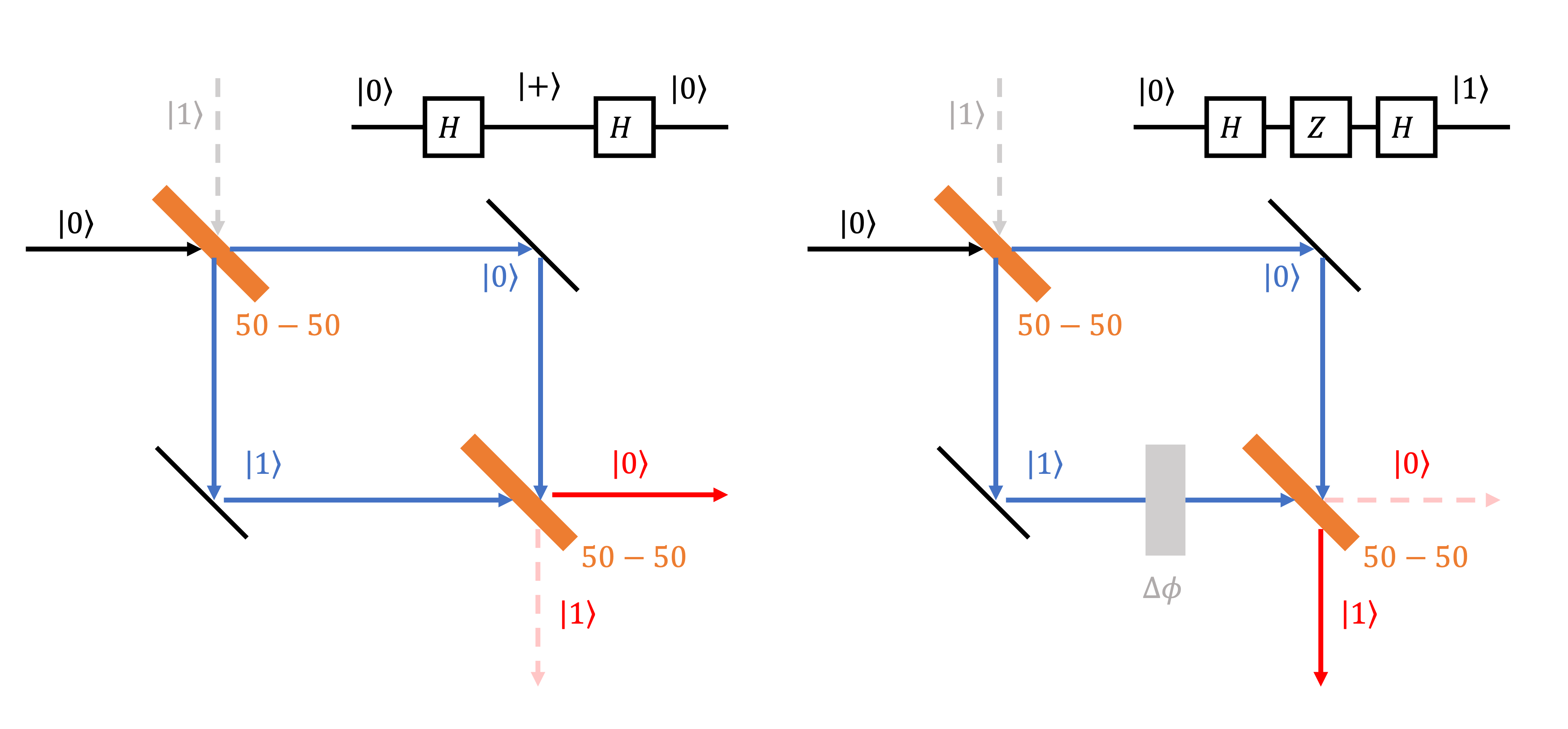
A qubit in \(\alpha|0\rangle+\beta|1\rangle\) is not a store of many answers. Measurement returns one bit, and never both amplitudes.
What it does add is a second path. Like the two arms of an interferometer, the amplitudes can be shifted in phase and then brought back together, so the outcome you want adds up and the others cancel.
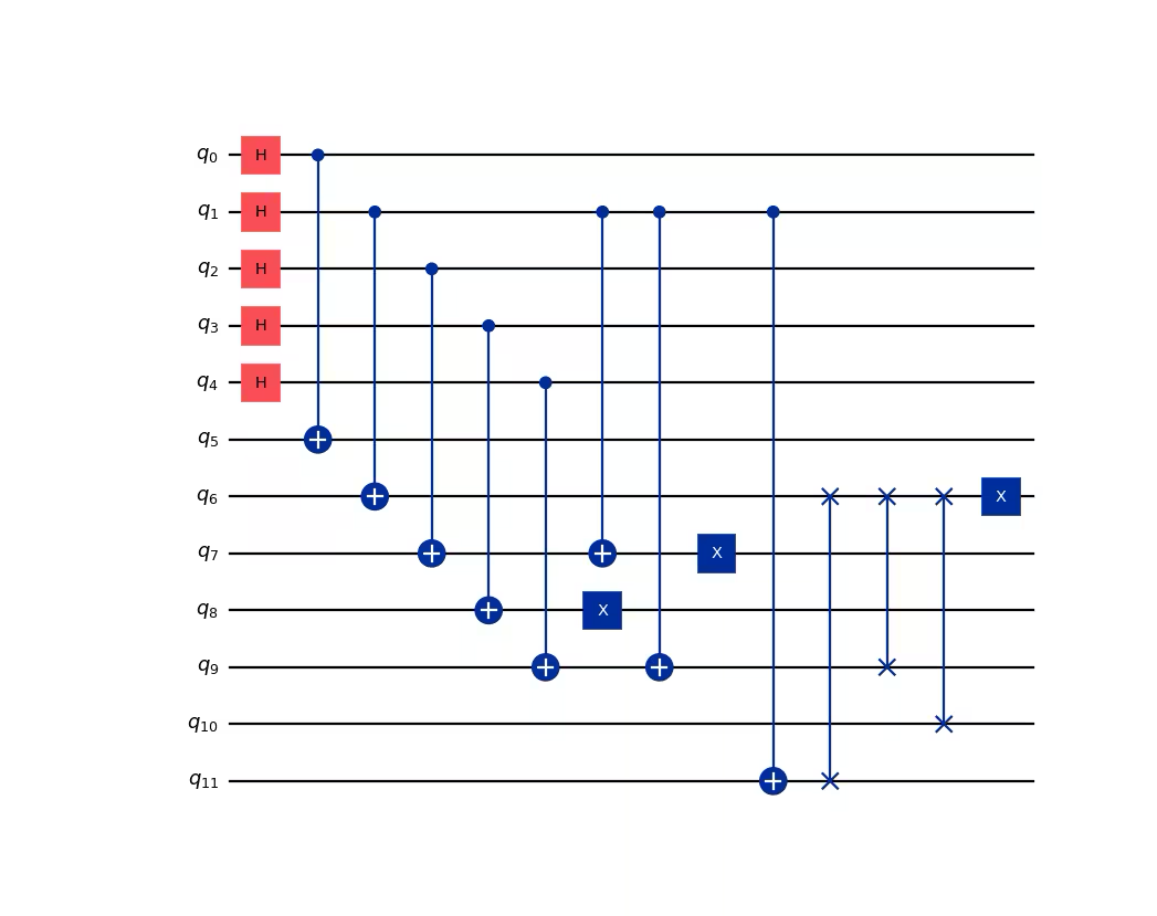
\[|0\rangle\xrightarrow{H}\frac{|0\rangle+|1\rangle}{\sqrt2} \xrightarrow{Z}\frac{|0\rangle-|1\rangle}{\sqrt2} \xrightarrow{H}|1\rangle.\]
\[\boxed{\text{superposition}+\text{phase control} +\text{interference}+\text{measurement}.}\]
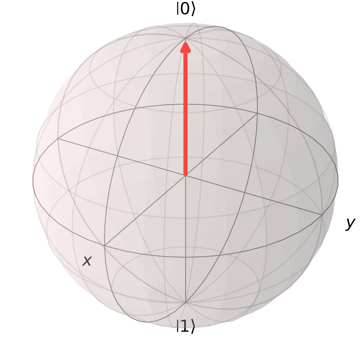
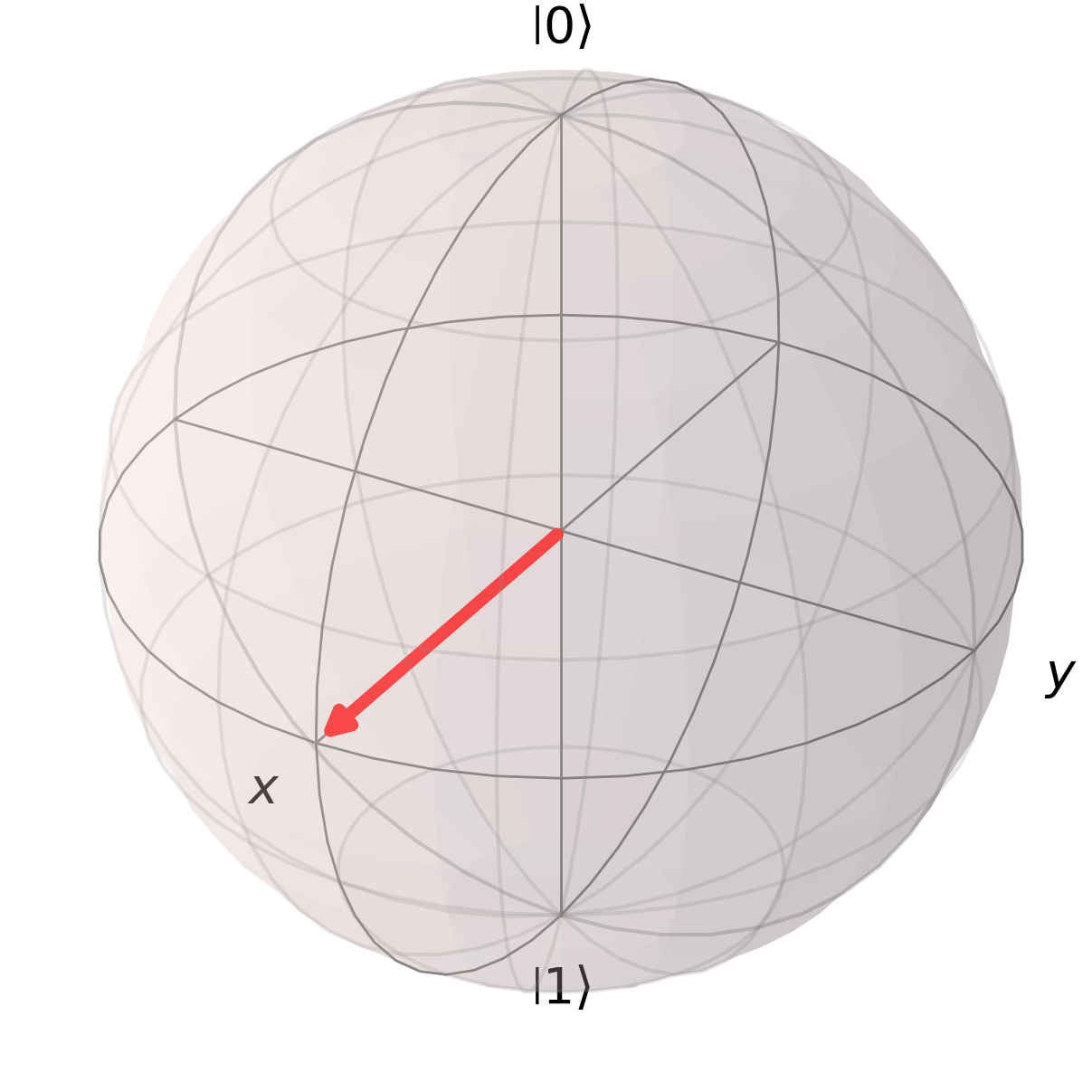
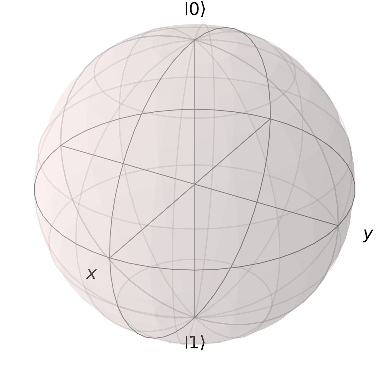
Question: After the CNOT entangles \(A\) and \(B\), how should the two qubits be drawn?
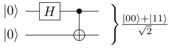
Entanglement.
\(|0_A\rangle |0_B\rangle\xrightarrow{H\otimes I} \left(\frac{|0_A\rangle+|1_A\rangle }{\sqrt2}\right)|0_B\rangle \xrightarrow{\mathrm{CNOT}} \frac{|0_A\rangle |0_B\rangle+|1_A\rangle |1_B\rangle}{\sqrt2}\)
Initial
After \(H_A\)
After CNOT
\(A\)
\(B\)
Q3. What Can a Machine Compute?
Computability, Complexity, and Universality
Interactive One-Bit Arithmetic Machine (Turing-Machine-Inspired)
Type directly on the tape. The start marker is #; the next two cells accept 0 or 1; the
following cell accepts + or *. Then press Run. The head reads
+ and follows the addition/half-adder path; it reads * and follows the
binary multiplication (AND) path.
Current stateqStart
Head actionRead
Read symbol1
Remembered bitsA=— ·
B=— · OUT=—
Step / result0 /
—
Half-adder circuit
qStartReada=□ · b=□▼
9 named control states
qStart, qReadA, qReadB, qReadOp, qAdd, qMul, qWrite, qReturn, qHalt
This compact teaching machine has 9 named control states. It shows every Read, Write, Move Left, Move Right, and Halt action; after writing the result, the head returns to #.
Universal Turing Machine
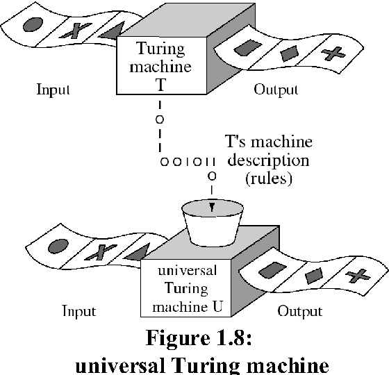
Turing machine \(M\) and input \(x\): \(M(x)\)
\(M\) has its own fixed rules. It runs on \(x\) and gives \(M(x)\).
Universal Turing machine \(U\)
\(U\) reads the description \(\langle M\rangle\) of \(M\), so \(U\) can simulate \(M\).
\[U(\langle M\rangle,x)=M(x)\]
The rules of \(U\) never change. The machine being simulated is data on the tape.
Universal does not mean simultaneous or fast. It means that an encoding exists and the fixed machine can reproduce the other machine's computation, possibly with overhead.
Computability and Complexity
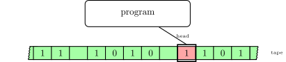
Computable
An algorithm gives the correct output and halts after finitely many steps for every valid input.
Decidable
For a yes/no problem, an algorithm halts with the correct answer on every input.
Undecidable
The Halting Problem has no algorithm that correctly answers every program–input pair.
Once an algorithm halts, how much does it cost?
Let \(n\) denote input size. Complexity records how required resources scale with \(n\).
Time
Sequential steps or circuit depth; independent operations may share one layer.
Space
Maximum working storage used at once: bits, qubits, or tape cells.
Operations
Total elementary operations, gates, or oracle queries in the chosen cost model.
Complexity is a scaling law—not merely a stopwatch measurement.
Feynman's Question: Can Nature Efficiently Simulate Itself?
An arbitrary pure state of (n) two-level systems is
\[|\psi\rangle=\sum_{x\in\{0,1\}^n}\alpha_x|x\rangle,\qquad \sum_x|\alpha_x|^2=1.\]
A direct classical description contains \(2^n\) complex amplitudes. This does not prove that every quantum system is classically hard to simulate—structure, symmetry, sparsity, and approximation can help—but it identifies a serious scaling problem for generic many-body dynamics.
Feynman's proposal reverses the strategy: rather than forcing a classical machine to track every amplitude, construct a controllable quantum system whose own evolution represents the target dynamics.
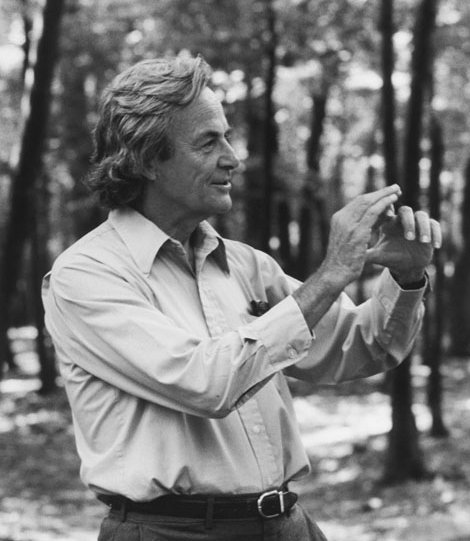
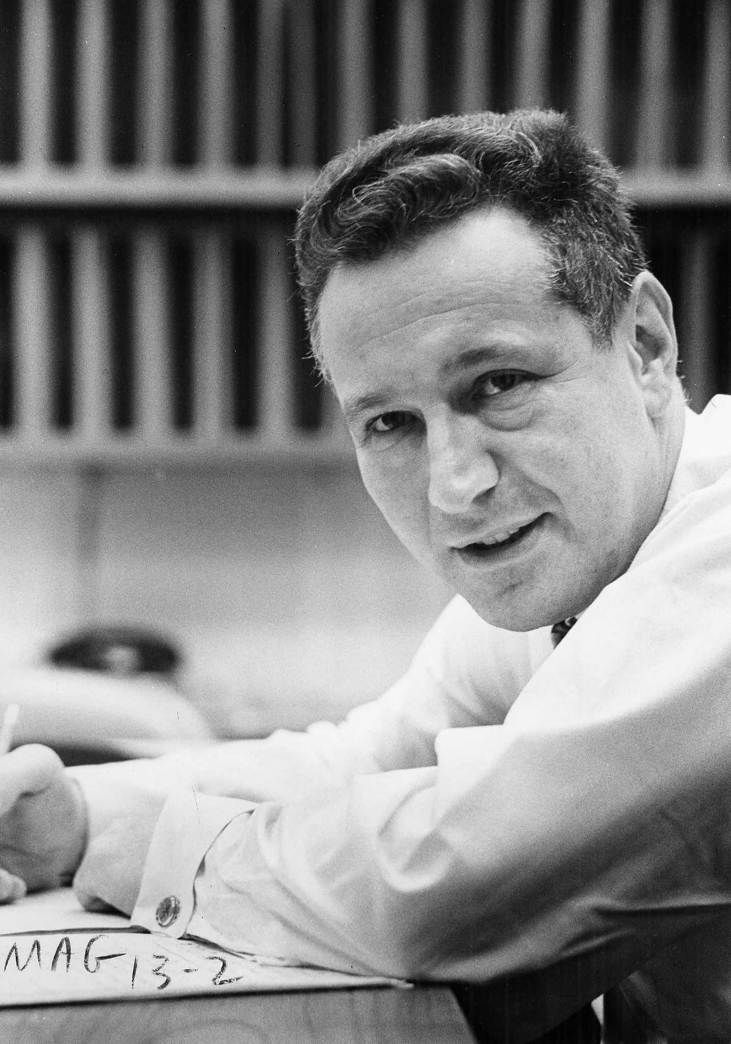
Richard Feynman
Ref:
Wikipedia
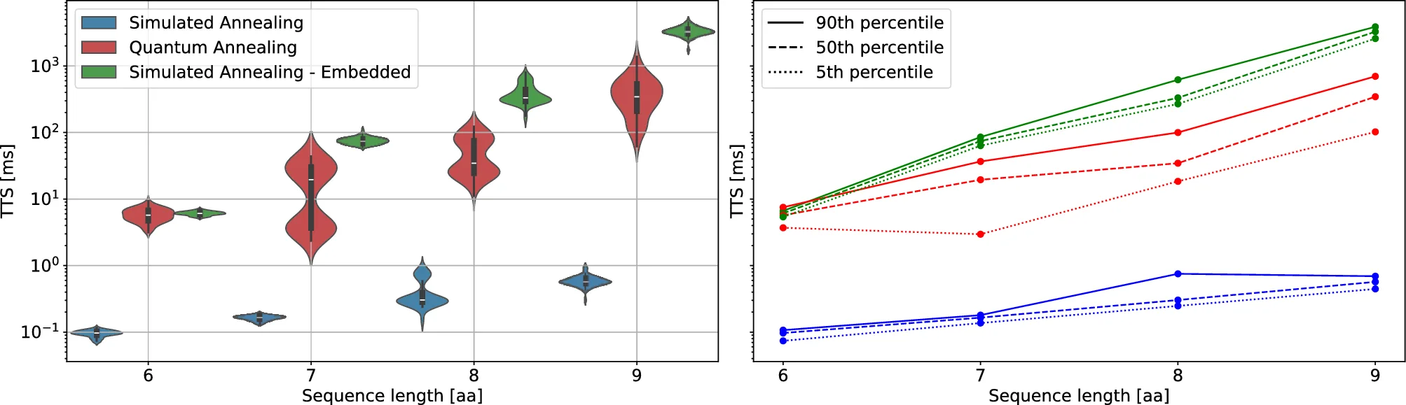
Protein Folding: Quantum Annealing vs. GPU Simulated Annealing
Independent quantum and classical solvers on the same protein-folding instances
Quantum hardware
D-Wave Advantage 2 prototype · Zephyr · about 1,200 device qubits
\(N=6\)–\(9\): up to 377 physical qubits after embedding
Anneal time: \(150~\mu\mathrm{s}\)
Classical hardware
2 × NVIDIA A100 GPUs
432 independent SA instances run in parallel.
Solver: graph-coloured multi-spin GPU-SA.
Reported \(\tau\) includes this GPU parallelism.
Measured quantities
Measured: \(p_{\mathrm{ground}},\ \tau,\ \mathrm{TTS}_{99\%}\)
\[\mathrm{TTS}_{99\%}=\tau\, \frac{\ln(1-0.99)}{\ln(1-p_{\mathrm{ground}})}\]
Timing boundary: QA \(\tau\) is anneal time. SA \(\tau\) is sampling time. Graph colouring is excluded.
Result: Original logical QUBO—GPU-SA is faster by orders of magnitude. Same embedded QUBO—QA is faster than this GPU-SA implementation. No scaling advantage is claimed.
Three Molecules Sampled on an IBM Heron QPU
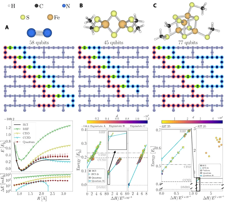
\(N_2\)breaking the triple bond · 58 qubits
[2Fe–2S]iron–sulfur cluster · 45 qubits
[4Fe–4S]larger cluster · 77 qubits
What they did
The Heron QPU never computes an energy. It samples electronic configurations — which orbitals are occupied. Fugaku then takes the configurations that came back, builds a small subspace out of them, and diagonalizes that classically. This is sample-based quantum diagonalization.
What came out
The \(N_2\) curve stays close to the reference right through bond breaking, where restricted CCSD falls apart. For the iron–sulfur clusters, hardware samples gave lower energies than uniformly random ones at the same subspace size — chemical signal survived a deep, noisy circuit.
Still a demonstration, not a quantum advantage. The paper claims no end-to-end speedup, and on the largest case — [4Fe–4S] at 77 qubits — leading classical methods still produced better solutions. What it shows is that a noisy QPU can be a useful sampler inside a classical workflow.
Shor's Shock: Quantum Advantage Is Not Limited to Simulating Physics
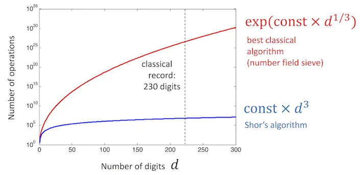
Integer factoring is computable on a classical computer. Shor's algorithm did not change its computability; it changed the known asymptotic resource scaling by exploiting quantum period finding.
\[\text{same problem}+\text{different physical model of computation}\Rightarrow\text{different complexity}.\]
This makes a stronger claim than “quantum systems simulate quantum systems”: superposition, phase, interference, and entanglement may reorganize the cost of tasks stated in ordinary mathematical language.
Avoid saying that Shor proves all quantum computers are faster. Speedup is problem- and algorithm-dependent, and practical advantage also includes error correction and hardware overhead.
Peter Shor
Ref:
Wikipedia
Why Shor's Algorithm Threatens RSA
RSA publishes \(N=pq\), the product of two large secret primes. Multiplying is easy; recovering \(p\) and \(q\) from \(N\) is believed to be extremely costly classically — and once you have them, the private key follows.
Shor's key step: turn factoring into period finding, which a large fault-tolerant quantum computer does in polynomial time.
Keys in use today
2048 bits
\(\approx617\) decimal digits. NIST wants 3072 bits beyond 2030. The classical record is RSA-250 — only 250 digits, in 2020.
Perfect qubits Shor needs
\(\sim\)4,100 logical
About \(2n+3\) for an \(n\)-bit modulus. These are idealised, error-free qubits — nobody has one.
After error correction
\(10^{6}\)–\(10^{7}\) physical
The surface code spends thousands of physical qubits per logical one: 20 million qubits / 8 hours (Gidney & Ekerå 2021), cut to under 1 million / a few days by 2025.
Prototypes today
\(10^{2}\)–\(10^{3}\) physical
IBM Heron 156, Google Willow 105, IBM Condor 1,121 — all noisy, none fault-tolerant. Roughly four orders of magnitude short.
Shor's Algorithm as a Pipeline
- Reduce factoring \(N\) to finding the order \(r\) of \(a\bmod N\).
- Create a coherent superposition of exponents.
- Compute modular exponentiation reversibly.
- Use phase estimation / the quantum Fourier transform to extract information about \(r\).
- Apply continued fractions and classical number theory to recover factors.
The quantum computer does not simply “try every factor.” Its advantage comes from encoding periodic structure into phase and extracting that structure through interference.
The modular-arithmetic circuit, not the textbook QFT diagram alone, dominates much of the logical resource cost.
Question: Gate-Based vs. Adiabatic Quantum Computing
Gate-Based / Circuit Model








Adiabatic Evolution / Quantum Annealing