Week 6 · Two-Qubit Interactions

PHYS598500 · Week 6

Two-Qubit Interactions

This week and next: one coupling

A coupling \(g\) connects a transmon to a partner. The two weeks use the same matrix and the same AC Stark shift.

	This week: two-qubit gate	Next week: readout
partner	a second transmon, \(\alpha_2\neq0\)	a resonator, \(\alpha_2=0\); then \(\zeta=2\chi\)
use	CZ: the phase stays in the qubits	readout: the photons leave at the rate \(\kappa\) and go to the amplifier

PHYS598500 · Week 6

Two-qubit gates

Universal gates: classical logic first

1 · NAND

\(a\)	\(b\)	\(\mathrm{NAND}\)
0	0	1
0	1	1
1	0	1
1	1	0

NAND gates can make every Boolean function:

\[\begin{aligned}\mathrm{NOT}\,a&=\mathrm{NAND}(a,a)\\a\ \mathrm{AND}\ b&=\mathrm{NOT}\,\mathrm{NAND}(a,b)\end{aligned}\]

NAND is not reversible.

2 · CCNOT (Toffoli)

\(a\)	\(b\)	\(c\)	\(c\oplus ab\)
0	0	0	0
0	0	1	1
0	1	0	0
0	1	1	1
1	0	0	0
1	0	1	1
1	1	0	1
1	1	1	0

\[\mathrm{CCNOT}(a,b,c)=(a,\,b,\,c\oplus ab)\]

CCNOT flips \(c\) only when \(a=b=1\). CCNOT is reversible, as each quantum gate must be.

3 · Set \(c=1\)

\(a\)	\(b\)	\(1\oplus ab\)
0	0	1
0	1	1
1	0	1
1	1	0

\[1\oplus ab=\mathrm{NAND}(a,b)\]

Thus a reversible gate can do all classical logic.

M. A. Nielsen and I. L. Chuang, Quantum Computation and Quantum Information (Cambridge, 2010), Sec. 1.4.1 and 3.2.5.

Why a two-qubit gate

Gate set \(\{\mathrm{CNOT},H,T\}\), with \(T=\mathrm{diag}(1,e^{i\frac{\pi}{4}})\). For each \(n\)-qubit unitary \(U\) and each \(\varepsilon>0\), can a finite circuit \(V\) of these gates give

\[\min_{\phi}\left\|U-e^{i\phi}V\right\|<\varepsilon\ ?\]

Yes. This property is universality. The phase \(e^{i\phi}\) is a global phase and has no physical effect. Any entangling two-qubit gate can replace CNOT: the hardware uses CZ or iSWAP.

M. A. Nielsen and I. L. Chuang, Quantum Computation and Quantum Information (Cambridge, 2010), Sec. 4.5.

H gate: physical Z and virtual Z

\(H=i\,R_z(\tfrac{\pi}{2})\,R_x(\tfrac{\pi}{2})\,R_z(\tfrac{\pi}{2}),\qquad R_\phi(\tfrac{\pi}{2})\,R_z(\theta)=R_z(\theta)\,R_{\phi-\theta}(\tfrac{\pi}{2})\)

Physical Z: two flux pulses

Virtual Z: two frame updates

LO (never changes) \(I(t)\) \(Q(t)\) flux \(\delta\omega_{01}(t)\) \(V_{\rm RF}(t)\) The carrier has fewer cycles than the real signal.

Virtual-Z theory: D. C. McKay et al., Phys. Rev. A 96, 022330 (2017), Sec. I. Lecture animation of an ideal two-state evolution.

H gate: physical Z and virtual Z on the Bloch sphere

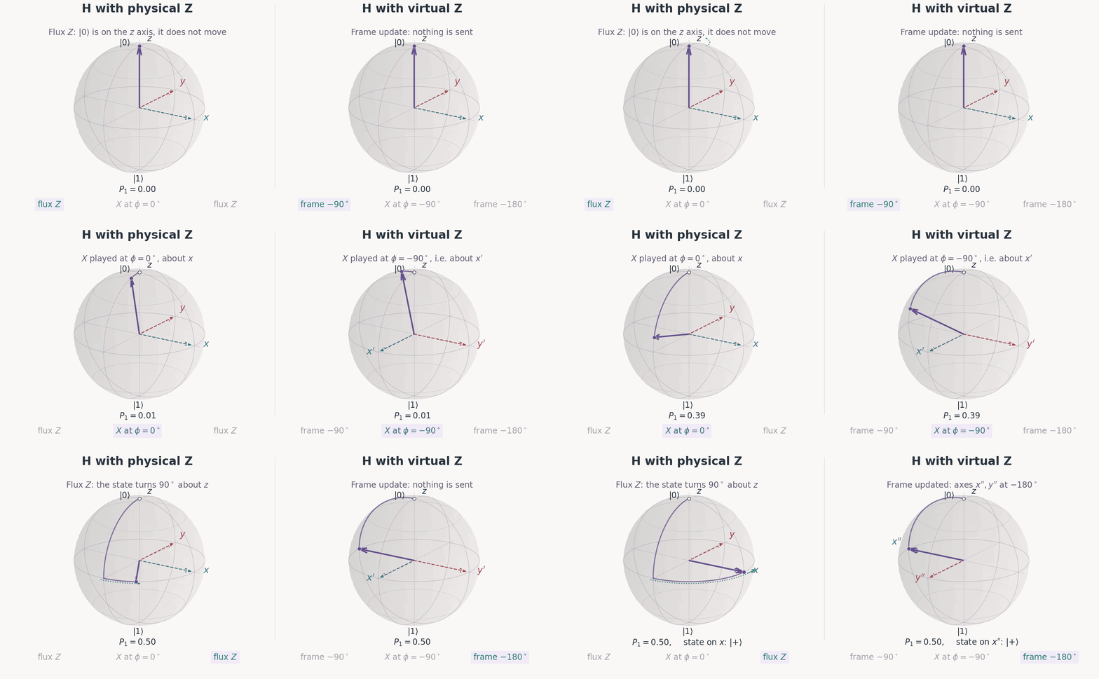
Two Bloch spheres, input |0⟩. Left, H with physical Z: a flux Z leaves |0⟩ in place, an X at phase 0 turns it to minus y, a second flux Z turns it to plus x. Right, H with virtual Z: the axes blink and jump to x′, y′ at minus 90 degrees, an X played at phase minus 90 degrees turns |0⟩ to minus x, the axes blink and jump to x″, y″ at minus 180 degrees, so the state lies on x″. Both end with P1 = 0.50, the state |+⟩.

Lecture simulation of an ideal two-state evolution with a fixed drive reference.

H gate: where the signals go

H by input

Single transmon chip: qubit drive line from the top, flux bias line from the right, readout resonator and readout input and output lines on the left

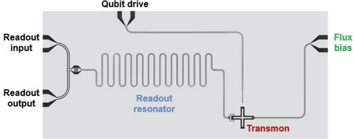
Circuit image: T. E. Roth et al., arXiv:2106.11352; it only shows the signal lines. Lecture animation of an ideal two-state evolution. The carrier has fewer cycles than the real signal.

Single-qubit gates: T and S

\[T=\begin{pmatrix}1&0\\0&e^{i\frac{\pi}{4}}\end{pmatrix}=e^{i\frac{\pi}{8}}R_z\big(\tfrac{\pi}{4}\big),\qquad S=\begin{pmatrix}1&0\\0&i\end{pmatrix}=e^{i\frac{\pi}{4}}R_z\big(\tfrac{\pi}{2}\big)\]

\[T^2=S,\qquad S^2=Z\]

T and S turn the state about \(z\) by 45° and 90°. The phase in front of each gate is a global phase. H needs one drive pulse and two turns about \(z\).

The equator of the Bloch sphere, seen from \(+z\).

T and S on the chip: physical or virtual

gate by input

Circuit image: T. E. Roth et al., arXiv:2106.11352; it only shows the signal lines. Lecture animation of an ideal two-state evolution. Virtual Z: D. C. McKay et al., Phys. Rev. A 96, 022330 (2017).

Four gates: matrix and truth table

The basis order is \(|00\rangle,|01\rangle,|10\rangle,|11\rangle\). The first label is qubit 1. Each row of the table is one column of the matrix: the output for that input.

\[\mathrm{CNOT}=\begin{pmatrix}1&0&0&0\\0&1&0&0\\0&0&0&1\\0&0&1&0\end{pmatrix}\]

in	out
\(\|00\rangle\)	\(\|00\rangle\)
\(\|01\rangle\)	\(\|01\rangle\)
\(\|10\rangle\)	\(\|11\rangle\)
\(\|11\rangle\)	\(\|10\rangle\)

CNOT applies X to qubit 2 when qubit 1 is in \(|1\rangle\).

\[\mathrm{CZ}=\begin{pmatrix}1&0&0&0\\0&1&0&0\\0&0&1&0\\0&0&0&-1\end{pmatrix}\]

in	out
\(\|00\rangle\)	\(\|00\rangle\)
\(\|01\rangle\)	\(\|01\rangle\)
\(\|10\rangle\)	\(\|10\rangle\)
\(\|11\rangle\)	\(-\|11\rangle\)

CZ puts \(-1\) on \(|11\rangle\) only.

\[\mathrm{iSWAP}=\begin{pmatrix}1&0&0&0\\0&0&i&0\\0&i&0&0\\0&0&0&1\end{pmatrix}\]

in	out
\(\|00\rangle\)	\(\|00\rangle\)
\(\|01\rangle\)	\(i\|10\rangle\)
\(\|10\rangle\)	\(i\|01\rangle\)
\(\|11\rangle\)	\(\|11\rangle\)

iSWAP exchanges \(|01\rangle\) and \(|10\rangle\) and adds the phase \(i\).

\[\mathrm{SWAP}=\begin{pmatrix}1&0&0&0\\0&0&1&0\\0&1&0&0\\0&0&0&1\end{pmatrix}\]

in	out
\(\|00\rangle\)	\(\|00\rangle\)
\(\|01\rangle\)	\(\|10\rangle\)
\(\|10\rangle\)	\(\|01\rangle\)
\(\|11\rangle\)	\(\|11\rangle\)

SWAP exchanges the states of the two qubits.

√iSWAP makes entanglement

\[\sqrt{\mathrm{iSWAP}}=\begin{pmatrix}1&0&0&0\\0&\tfrac{1}{\sqrt2}&\tfrac{i}{\sqrt2}&0\\0&\tfrac{i}{\sqrt2}&\tfrac{1}{\sqrt2}&0\\0&0&0&1\end{pmatrix},\qquad\big(\sqrt{\mathrm{iSWAP}}\big)^2=\mathrm{iSWAP}\]

Start in \(|10\rangle\):

\[\sqrt{\mathrm{iSWAP}}\,|10\rangle=\tfrac{1}{\sqrt2}\big(|10\rangle+i|01\rangle\big)\]

Product test: \(c_{00}c_{11}=0\), but \(c_{01}c_{10}=\tfrac{i}{2}\). The test fails, thus the state is entangled.

The full iSWAP changes \(|10\rangle\) to \(i|01\rangle\). This is a product state.

Compiling to CZ

A Hadamard gate on the target changes \(Z\) into \(X\), because \(HZH=X\):

\[(\mathbb 1\otimes H)\,\mathrm{CZ}\,(\mathbb 1\otimes H)=|0\rangle\langle0|\otimes\mathbb 1+|1\rangle\langle1|\otimes X=\mathrm{CNOT}\]

CZ is symmetric. It has no control qubit and no target qubit.

A SWAP is three CNOTs. The middle CNOT has its control on qubit 2: \(b\to a\oplus b\), then \(a\to b\), then \(a\oplus b\to a\).

On a CZ machine, a SWAP costs three CZ gates.

Compiling to iSWAP

A CNOT costs two iSWAPs and three single-qubit gates. \(S^\dagger\) is a virtual Z gate.

\[\mathrm{iSWAP}=(S\otimes S)\,\mathrm{CZ}\,\mathrm{SWAP},\qquad S=\mathrm{diag}(1,i)\]

An iSWAP is a SWAP with a CZ and two S gates. Thus \(\mathrm{SWAP}=(S^\dagger\otimes S^\dagger)\,\mathrm{CZ}\,\mathrm{iSWAP}\).

All circuits are correct up to a global phase.

N. Schuch and J. Siewert, Phys. Rev. A 67, 032301 (2003).

CCNOT from CNOTs and T gates

On a CZ machine, each CNOT is one CZ and two H gates: six CZ gates. The T gates are virtual Z gates.

With \(c=1\), the output on \(c\) is \(\mathrm{NAND}(a,b)\). Thus a processor with these gates can also run all classical logic.

M. A. Nielsen and I. L. Chuang, Quantum Computation and Quantum Information (Cambridge, 2010), Fig. 4.9.

Native gates

A native gate is the two-qubit gate that the hardware makes directly from its Hamiltonian. The compiler makes all other gates from the native gate and single-qubit gates.

What the hardware does	Native gate	Example
A flux pulse moves Q1 until \(\|11\rangle\) meets \(\|20\rangle\)	CZ	Google Willow; IBM Heron (tunable coupler)
A flux pulse moves Q1 until \(\|01\rangle\) meets \(\|10\rangle\)	iSWAP-type	Google Sycamore
A microwave drive on Q1 at the frequency of Q2	Cross-resonance	IBM Eagle (fixed frequencies)

F. Arute et al., Nature 574, 505 (2019) · Google Quantum AI, Nature 638, 920 (2025).

Native gates across qubit types

Qubit	What couples two qubits	Native gate	Switched by	Time	Best reported
Transmon, tunable Google; IBM Heron	capacitor \(g\) (or a tunable coupler)	CZ (\(\|11\rangle\leftrightarrow\|20\rangle\)); iSWAP-type	flux pulse	tens of ns	CZ 99.76 %, 60 ns ¹
Transmon, fixed IBM Eagle	capacitor \(g\)	cross-resonance, CNOT	microwave drive on Q1 at \(\omega_2\)	100s of ns	CNOT 99.77 %, 180 ns ²
Fluxonium	capacitor (+ transmon coupler)	CZ, microwave-activated via non-computational levels	microwave drive	~100 ns	CZ 99.85–99.9 % ³
Trapped ions Quantinuum, IonQ	shared motion of the ion chain	Mølmer–Sørensen XX (or a ZZ phase gate)	laser (or microwave) pulse	10–100 μs	99.9 % ⁴
Neutral atoms QuEra, Atom Computing	Rydberg blockade	CZ (also CCZ)	laser to the Rydberg state	sub-μs	CZ 99.5 %, 60 atoms in parallel ⁵
Spins in silicon quantum dots	exchange \(J\) (overlap of the electrons)	CZ, CPhase (or \(\sqrt{\mathrm{SWAP}}\))	gate voltage on the barrier	~100 ns	CZ > 99.5 % ⁶
Photons PsiQuantum	no direct interaction; interference + detection	fusion (a Bell measurement), probabilistic, heralded	detection (heralded)	—	fusion 99.22 % (conditional on detection) ⁷

Superconducting qubits and spin qubits have ns gates and connect only to their nearest neighbours. Ions and atoms have slower gates, but they can connect any pair.

¹ Y. Sung et al., Phys. Rev. X 11, 021058 (2021) · ² A. Kandala et al., Phys. Rev. Lett. 127, 130501 (2021) · ³ L. Ding et al., Phys. Rev. X 13, 031035 (2023) · ⁴ C. J. Ballance et al., Phys. Rev. Lett. 117, 060504 (2016) · ⁵ S. J. Evered et al., Nature 622, 268 (2023) · ⁶ X. Xue et al., Nature 601, 343 (2022) · ⁷ PsiQuantum team, Nature 641, 876 (2025).

PHYS598500 · Week 6

Coupling

Fixed or tunable: four designs

Fixed qubits, fixed \(g\)

Control: Cross-resonance, a drive on Q1 at \(\omega_2\).

+ Fewest lines. No flux noise.

− Static ZZ. Frequency crowding. Slow gates.

Tunable qubits, fixed \(g\)

Control: Flux moves Q1 to a resonance (iSWAP, CZ).

+ Fast gates. Flux avoids collisions.

− Static ZZ. Flux noise.

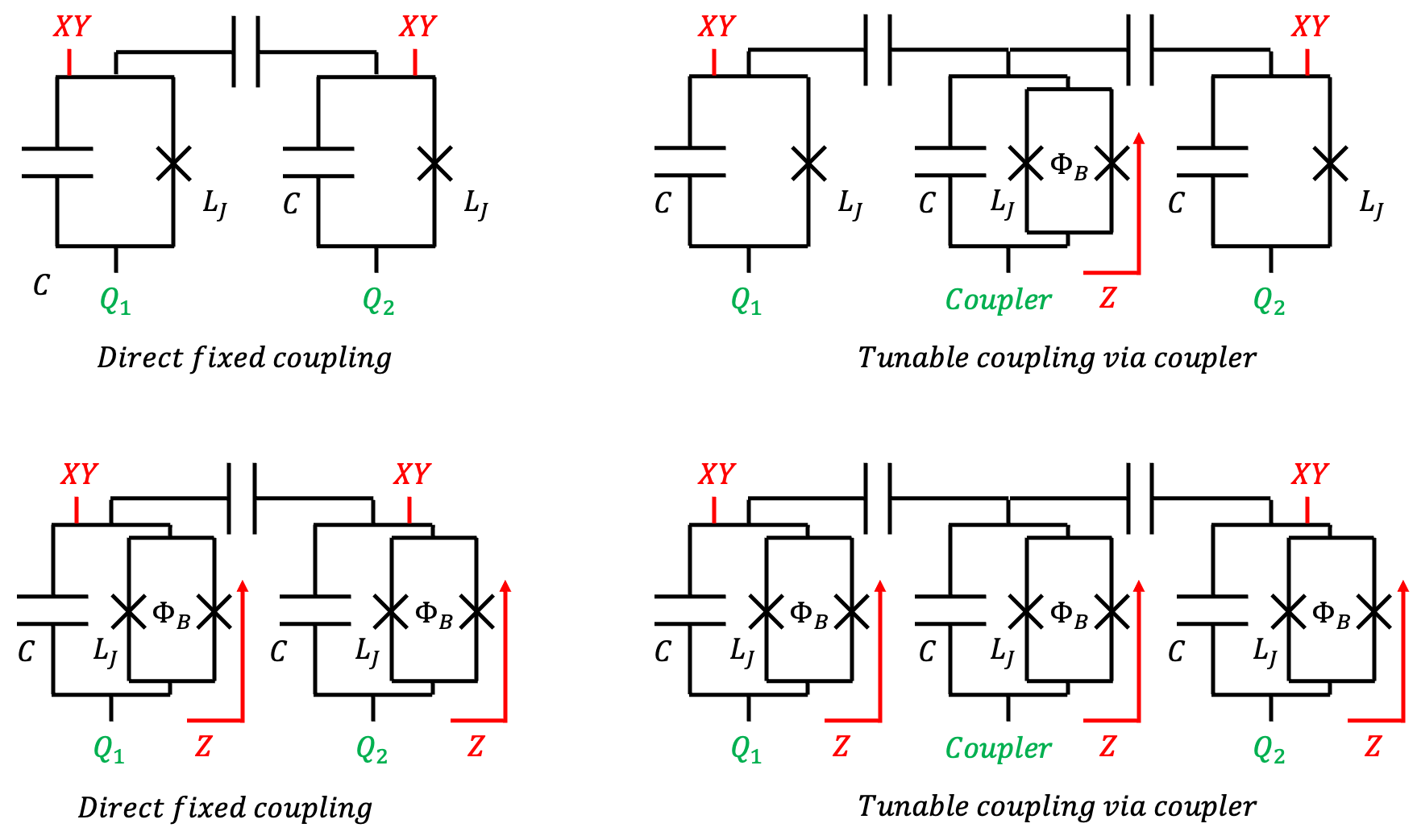
Four circuits. Top: fixed-frequency qubits (one junction, XY line only). Bottom: tunable-frequency qubits (two junctions with flux, XY and Z lines). Left: direct fixed coupling through one capacitor. Right: tunable coupling through a coupler with its own Z line

Fixed qubits, coupler

Control: Flux on the coupler turns ZZ on (CZ).

+ \(g_{\rm eff}\approx0\) at idle. No flux noise on the qubits.

− Frequency crowding.

Tunable qubits, coupler

Control: Flux on the qubits and the coupler (CZ, iSWAP).

+ \(g_{\rm eff}\approx0\) at idle. Fast gates.

− Most lines. Flux noise.

IBM

Public family	Public year	Qubits	Qubit type	Qubit frequency tunable	Coupler tunable	Connectivity	Representative two-qubit control
Canary ^1,2,3,4	2016 public-cloud launch; grouped in the 2016-2019 roadmap period	5 in the roadmap; later IBM documentation uses Canary for 5-to-16-qubit designs	Fixed-frequency superconducting transmon platform	No	No	Small early connectivity graphs	CR-based CX
Albatross ^2,4	2016-2019 roadmap period	16	Fixed-frequency superconducting transmon platform	No	No	—	CR-based CX
Penguin ^2,4	2018-2019	20	Fixed-frequency transmon	No	No	Square and bow-tie revisions before heavy hex	CR-based CX
53-qubit prototype ^2,4,5	2019	53	IBM fixed-frequency superconducting transmon platform	No	No	—	CR-based control
Falcon ^4,6,7	2020	27 operational qubits in the main family	Fixed-frequency transmon	No	No	Heavy hex; degree two or three	CR, compiled as CX or ECR
Hummingbird ^4,6,7	2020	65	Fixed-frequency transmon	No	No	Heavy hex	CR, compiled as CX or ECR
Eagle ^8,9	2021	127	Fixed-frequency transmon	No	No	Heavy hex	CR, compiled as ECR

¹ IBM 2016 launch · ² IBM roadmap archive · ³ IBM retired-family documentation · ⁴ IBM fixed-frequency/CR architecture · ⁵ IBM statement on its 53-qubit processor · ⁶ IBM 2020 roadmap · ⁷ IBM agile-hardware article · ⁸ IBM Eagle architecture article · ⁹ IBM Eagle CR-performance article

IBM

Public family	Public year	Qubits	Qubit type	Qubit frequency tunable	Coupler tunable	Connectivity	Representative two-qubit control
Egret ^1,2	2022	33	Fixed-frequency transmon	No	Yes	Multi-qubit tunable-coupler test platform	Coupler-activated CZ
Osprey ^1,3,4	2022	433	Fixed-frequency transmon	No	No	Scaled fixed-coupling IBM layout	CR
Condor ⁵	2023	1,121	Fixed-frequency transmon	No	No	Scaled CR architecture	CR
Heron r1 ^5,6	2023	133	Fixed-frequency transmon	No	Yes	Heavy hex	Coupler-activated CZ
Heron r2 and r3 ^6,7,8	2024-2025	156	Fixed-frequency transmon	No	Yes	Heavy hex	Coupler-activated CZ
Nighthawk r1 ^7,9,10	2025	120	Fixed-frequency transmon inherited from the Heron technology stack	No	Yes	Square lattice; four-degree connectivity; 218 couplers	Coupler-activated CZ
Nighthawk r2 ^7,10,11	2026	120 programmable qubits; 218 gate couplers; 120 reset elements	Fixed-frequency transmon inherited from the Heron technology stack	No	Yes	Square lattice	Coupler-activated CZ plus independent dissipative reset

¹ IBM retired-family documentation · ² Stehlik et al., tunable-coupler experiment · ³ IBM Osprey article · ⁴ IBM fixed-frequency/CR architecture · ⁵ IBM Condor and Heron article · ⁶ McKay et al., experimental benchmark · ⁷ IBM processor-type documentation · ⁸ IBM current hardware page · ⁹ IBM Nighthawk announcement · ¹⁰ IBM backend documentation · ¹¹ IBM Nighthawk r2 technical article

Google

Public family	Public year	Qubits	Qubit type	Qubit frequency tunable	Coupler tunable	Connectivity	Representative two-qubit control
Xmon five-qubit array ¹	2014	5	Planar Xmon transmon	Yes	No	Linear nearest neighbor	CZ by qubit-frequency tuning near the \|11⟩ to \|02⟩ interaction
gmon experiment ²	2014	2 in the reported unit cell	Xmon-derived gmon	Yes	Yes	Experimental two-qubit cell	Tunable interaction and adiabatic CZ
Xmon nine-qubit linear array ^3,4	2015	9	Planar Xmon transmon	Yes	No	Linear nearest neighbor	Frequency-pulsed CZ
Foxtail ⁵	Publicly shown in 2018	22	Xmon	Yes	—	Bilinear array	—
Bristlecone ^3,6	2018	72	Xmon-family transmon	Yes	No	Two-dimensional nearest-neighbor array	Same coupling, control, and readout scheme as the prior nine-qubit array
Sycamore ^7,8	2019	54 fabricated; 53 used in the 2019 experiment	Tunable transmon	Yes	Yes	Two-dimensional square-grid family; up to four neighbors	fSim and Sycamore gate; later service data also list square-root iSWAP
Sycamore service variants, including Sycamore23 and the Weber service configuration ^8,9	2020-2021	23 or up to 54	Tunable transmon	Yes	Yes	Subset or full Sycamore grid	Square-root iSWAP and Sycamore gate
Willow ^9,10,11	2024	105	Flux-tunable superconducting transmon	Yes	Yes	Square grid; average connectivity 3.47 and four-way typical	CZ

¹ Barends et al., Nature 2014 · ² Chen et al., arXiv:1402.7367 · ³ Kelly et al., Nature 2015 · ⁴ Google nine-qubit control description · ⁵ Google Foxtail article · ⁶ Google Bristlecone article · ⁷ Arute et al., Nature 2019 · ⁸ service datasheet · ⁹ Google Cirq device specifications · ¹⁰ Google Willow paper · ¹¹ Google architecture note

IBM images

IBM chip micrograph: four colored readout resonators D1 to D4 and S1 around the qubits

IBM Osprey QPU structure: qubit, readout and wiring layers

IBM topology evolution from Penguin v1 to Falcon r4, with the average qubit connectivity

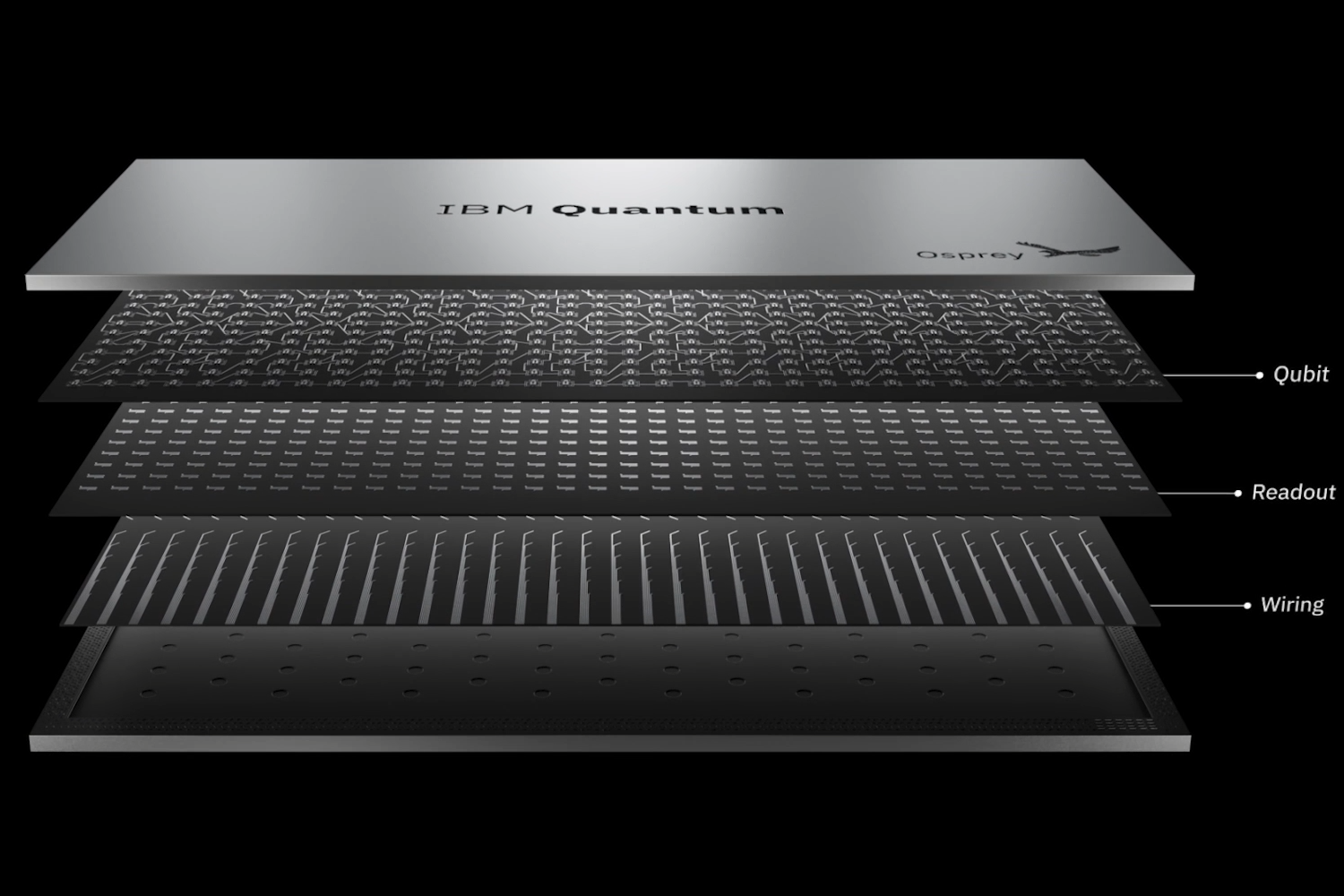
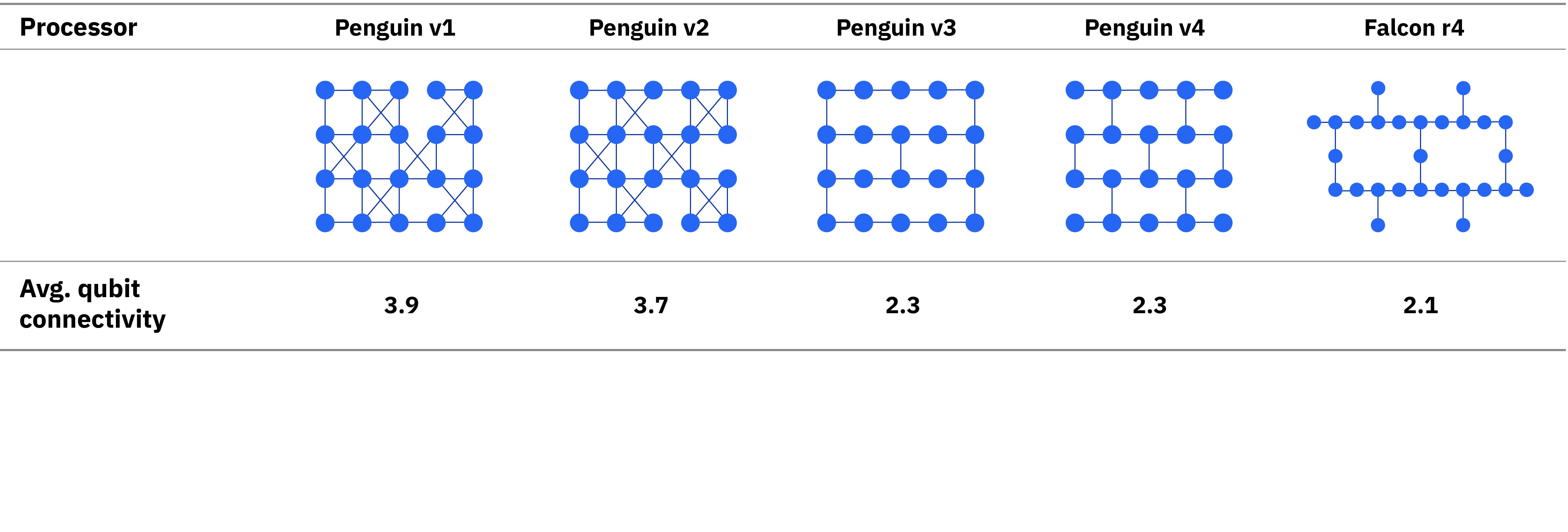
Left: M. Takita et al., Phys. Rev. Lett. 119, 180501 (2017), Fig. 1(a). Top right: Notebookcheck, “IBM announces 433-qubit quantum processor” (2022); image: IBM. Bottom right: P. Nation et al., “The IBM Quantum heavy hex lattice”, IBM Quantum blog (2021), Fig. 2.

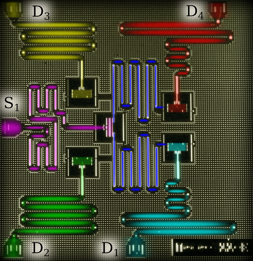
Google images

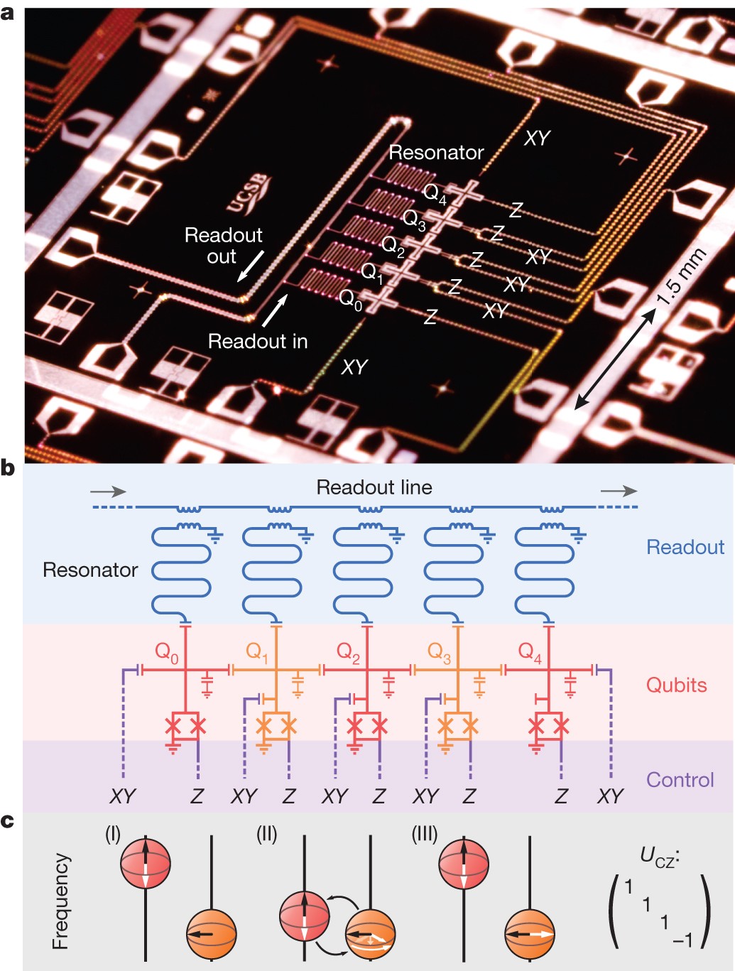
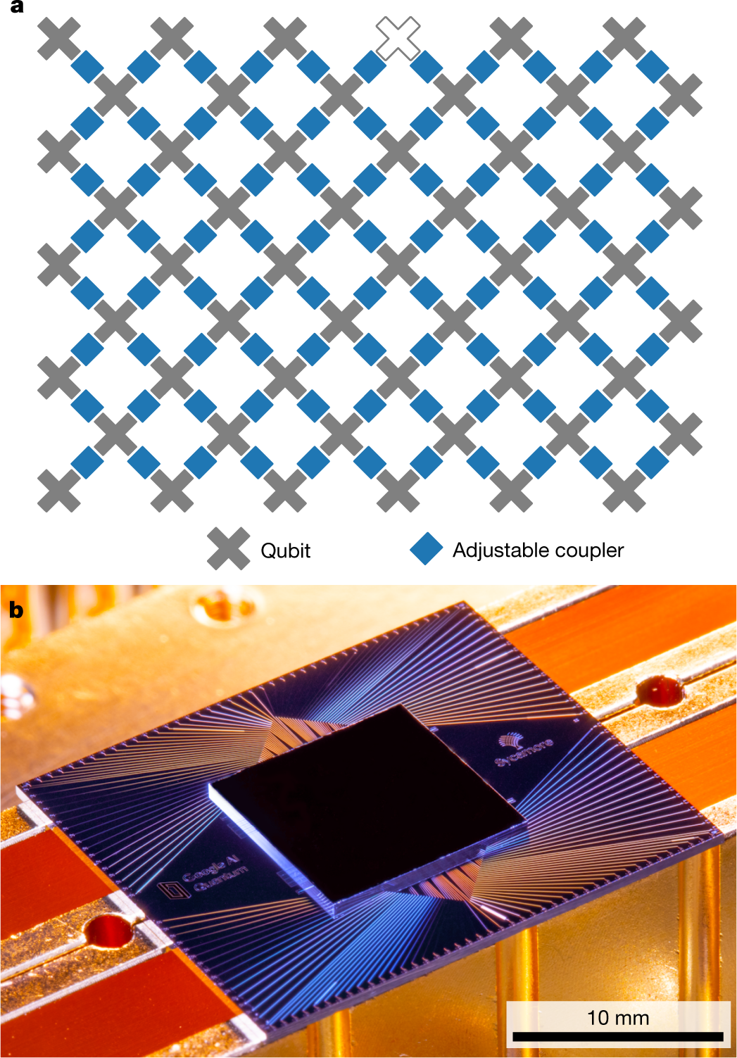
Left: R. Barends et al., Nature 508, 500 (2014), Fig. 1. Right: F. Arute et al., Nature 574, 505 (2019), Fig. 1.

Google images

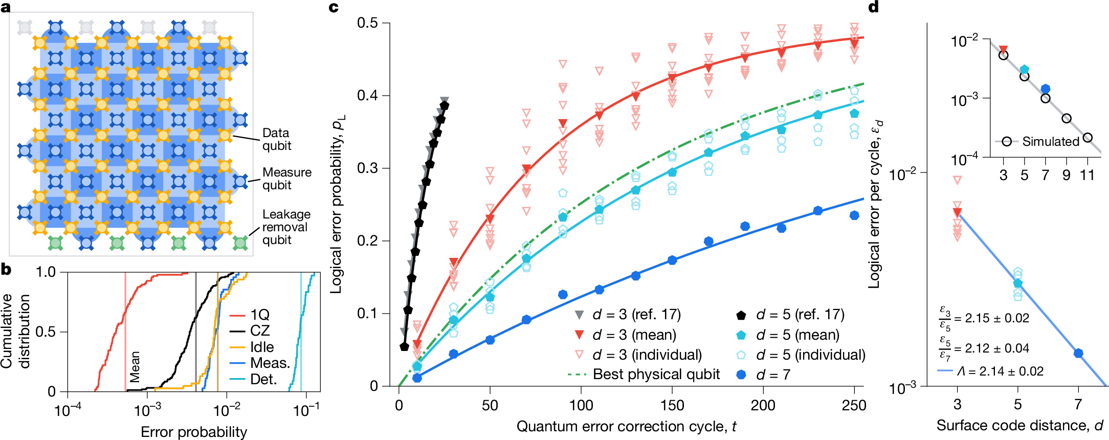
Willow surface-code architecture: 105-qubit square grid with distance-3, 5 and 7 regions

Google Quantum AI, Nature 638, 920 (2025), Fig. 1.

2D-array chip micrographs

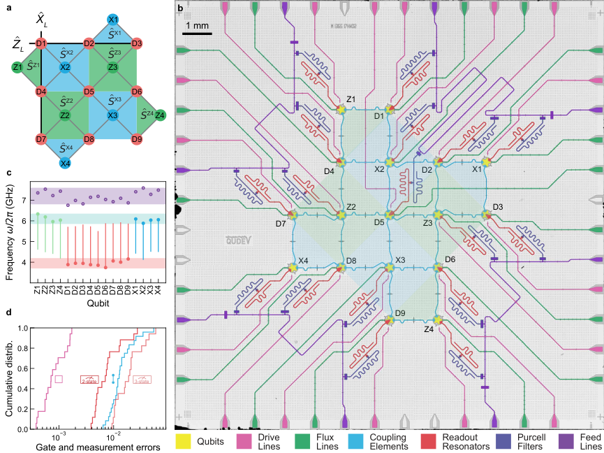
17 transmons in a 2D surface-code lattice (ETH); the micrograph is panel b

S. Krinner et al., Nature 605, 669 (2022), Fig. 1.

A coupling capacitor: the Lagrangian

The voltage on each capacitor, with ground at 0, is:

\[V_{C_1}=V_1,\qquad V_{C_2}=V_2,\qquad V_{C_g}=V_1-V_2\]

The junction phases obey \(\dot\varphi_j=\frac{2eV_j}{\hbar}\). The junction energy is \(U_J=-E_{J1}\cos\varphi_1-E_{J2}\cos\varphi_2\).

\[T=\frac12C_1V_1^2+\frac12C_2V_2^2+\frac12C_g\left(V_1-V_2\right)^2\]

The Lagrangian is \(\mathcal L=T-U_J\). Expand the \(C_g\) term:

\[\begin{aligned}\mathcal L&=\frac12\left(C_1+C_g\right)V_1^2+\frac12\left(C_2+C_g\right)V_2^2-C_gV_1V_2\\&\quad{}+E_{J1}\cos\varphi_1+E_{J2}\cos\varphi_2\end{aligned}\]

Substitute \(V_j=\frac{\hbar}{2e}\,\dot\varphi_j\):

\[\begin{aligned}\mathcal L(\varphi,\dot\varphi)&=\left(\frac{\hbar}{2e}\right)^2\Big[\frac12\left(C_1+C_g\right)\dot\varphi_1^2+\frac12\left(C_2+C_g\right)\dot\varphi_2^2\\&\qquad{}-C_g\,\dot\varphi_1\dot\varphi_2\Big]+E_{J1}\cos\varphi_1+E_{J2}\cos\varphi_2\end{aligned}\]

A coupling capacitor: the Hamiltonian

The conjugate momenta, with \(p=\hbar n\), are:

\[p_1=\frac{\partial\mathcal L}{\partial\dot\varphi_1}=\frac{\hbar}{2e}\Big[\left(C_1+C_g\right)V_1-C_gV_2\Big]=\hbar n_1\]

\[p_2=\frac{\partial\mathcal L}{\partial\dot\varphi_2}=\frac{\hbar}{2e}\Big[\left(C_2+C_g\right)V_2-C_gV_1\Big]=\hbar n_2\]

Write them as a matrix. Then solve exactly for the voltages:

\[2e\begin{pmatrix}n_1\\n_2\end{pmatrix}=\begin{pmatrix}C_1+C_g&-C_g\\-C_g&C_2+C_g\end{pmatrix}\begin{pmatrix}V_1\\V_2\end{pmatrix}\]

\[\begin{pmatrix}V_1\\V_2\end{pmatrix}=\frac{2e}{D}\begin{pmatrix}C_2+C_g&C_g\\C_g&C_1+C_g\end{pmatrix}\begin{pmatrix}n_1\\n_2\end{pmatrix}\]

\[D=C_1C_2+C_g\left(C_1+C_2\right)\]

The Hamiltonian is \(\mathcal H=p_1\dot\varphi_1+p_2\dot\varphi_2-\mathcal L=T+U_J\). Write the voltages with \(n_1\) and \(n_2\):

\[\mathcal H=4E_{C1}n_1^2-E_{J1}\cos\varphi_1+4E_{C2}n_2^2-E_{J2}\cos\varphi_2+\mathcal H_c\]

\[E_{C1}=\frac{e^2\left(C_2+C_g\right)}{2D},\qquad E_{C2}=\frac{e^2\left(C_1+C_g\right)}{2D}\]

\[\mathcal H_c=4e^2\,\frac{C_g}{D}\,n_1n_2\]

Use \(n=\tfrac{i}{2}\big(\tfrac{E_J}{2E_C}\big)^{\frac{1}{4}}(a^\dagger-a)\) and \(\hbar\omega_p=\sqrt{8E_JE_C}\):

\[\frac{\mathcal H_c}{\hbar}=-g\,(a_1^\dagger-a_1)(a_2^\dagger-a_2)\]

\[g=\frac{C_g\sqrt{\omega_{p1}\,\omega_{p2}}}{2\sqrt{\left(C_1+C_g\right)\left(C_2+C_g\right)}}\]

For \(C_g=0.32\) fF, \(C_1=C_2=80\) fF and \(\omega_p=2\pi\times5\) GHz, \(g\approx2\pi\times10\) MHz.

J. Koch et al., Phys. Rev. A 76, 042319 (2007).

Two transmons and one coupling

Each transmon is a ladder with its own \(\omega_1,\alpha_1\) and \(\omega_2,\alpha_2\):

\[\frac{\mathcal H}{\hbar}=\omega_1a_1^\dagger a_1+\frac{\alpha_1}{2}a_1^\dagger a_1^\dagger a_1a_1+\omega_2a_2^\dagger a_2+\frac{\alpha_2}{2}a_2^\dagger a_2^\dagger a_2a_2+\frac{\mathcal H_c}{\hbar}\]

The coupling capacitor gives:

\[\frac{\mathcal H_c}{\hbar}=-g\,(a_1^\dagger-a_1)(a_2^\dagger-a_2)\]

\[=g\,\big(a_1^\dagger a_2+a_1a_2^\dagger-a_1^\dagger a_2^\dagger-a_1a_2\big)\]

Rotate each transmon at its own frequency:

\[U=\sum_{j,k}e^{-i(j\omega_1+k\omega_2)t}\,|jk\rangle\langle jk|,\qquad\mathcal H_{\rm rot}=U^\dagger\mathcal H U-i\hbar\,U^\dagger\dot U\]

Each operator gets its own phase:

\[U^\dagger a_jU=a_j\,e^{-i\omega_jt},\qquad U^\dagger a_j^\dagger U=a_j^\dagger\,e^{i\omega_jt}\]

The term \(-i\hbar\,U^\dagger\dot U\) cancels the \(\omega_1\) and \(\omega_2\) terms. The \(\alpha\) terms do not turn. Keep all terms:

\[\begin{aligned}\frac{\mathcal H_{\rm rot}}{\hbar}&=\frac{\alpha_1}{2}a_1^\dagger a_1^\dagger a_1a_1+\frac{\alpha_2}{2}a_2^\dagger a_2^\dagger a_2a_2+g\,\big(e^{i\Delta t}a_1^\dagger a_2+e^{-i\Delta t}a_1a_2^\dagger\big)\\&\quad{}-g\,\big(e^{i(\omega_1+\omega_2)t}a_1^\dagger a_2^\dagger+e^{-i(\omega_1+\omega_2)t}a_1a_2\big)\end{aligned}\]

\(\Delta\equiv\omega_1-\omega_2\) is slow. \(\omega_1+\omega_2\approx2\pi\times10\) GHz is fast, and its average is zero (RWA):

\[\begin{aligned}\frac{\mathcal H_{\rm rot}}{\hbar}&\overset{\rm RWA}{\simeq}\frac{\alpha_1}{2}a_1^\dagger a_1^\dagger a_1a_1+\frac{\alpha_2}{2}a_2^\dagger a_2^\dagger a_2a_2\\&\quad{}+g\,\big(e^{i\Delta t}a_1^\dagger a_2+e^{-i\Delta t}a_1a_2^\dagger\big)\end{aligned}\]

Levels 0–2: one matrix for the week

This matrix uses levels 0–2 of each transmon. Blue shows levels 0 and 1 (the 4×4). Orange shows the couplings of level 2: \(|11\rangle\) has two partners, \(|20\rangle\) and \(|02\rangle\).

\[\frac{\mathcal H_{\rm rot}}{\hbar}:\quad\begin{array}{r|cccc|cc|ccc}&{\color{#6b6472}{|00\rangle}}&{\color{#6b6472}{|01\rangle}}&{\color{#6b6472}{|10\rangle}}&{\color{#6b6472}{|11\rangle}}&{\color{#6b6472}{|20\rangle}}&{\color{#6b6472}{|02\rangle}}&{\color{#6b6472}{|21\rangle}}&{\color{#6b6472}{|12\rangle}}&{\color{#6b6472}{|22\rangle}}\\\hline{\color{#6b6472}{|00\rangle}}&{\color{#355f9c}{0}}&&&&&&&&\\{\color{#6b6472}{|01\rangle}}&&{\color{#355f9c}{0}}&{\color{#355f9c}{g\,e^{-i\Delta t}}}&&&&&&\\{\color{#6b6472}{|10\rangle}}&&{\color{#355f9c}{g\,e^{i\Delta t}}}&{\color{#355f9c}{0}}&&&&&&\\{\color{#6b6472}{|11\rangle}}&&&&{\color{#355f9c}{0}}&{\color{#b5651d}{\sqrt2g\,e^{-i\Delta t}}}&{\color{#b5651d}{\sqrt2g\,e^{i\Delta t}}}&&&\\\hline{\color{#6b6472}{|20\rangle}}&&&&{\color{#b5651d}{\sqrt2g\,e^{i\Delta t}}}&{\color{#b5651d}{\alpha_1}}&&&&\\{\color{#6b6472}{|02\rangle}}&&&&{\color{#b5651d}{\sqrt2g\,e^{-i\Delta t}}}&&{\color{#b5651d}{\alpha_2}}&&&\\\hline{\color{#6b6472}{|21\rangle}}&&&&&&&\alpha_1&2g\,e^{i\Delta t}&\\{\color{#6b6472}{|12\rangle}}&&&&&&&2g\,e^{-i\Delta t}&\alpha_2&\\{\color{#6b6472}{|22\rangle}}&&&&&&&&&\alpha_1+\alpha_2\\\end{array}\]

The same matrix, drawn as levels

\(\Delta=\omega_1-\omega_2\) \(\alpha_1\) \(\alpha_2\)

Bare levels (\(g\to0\)). Each block is in its own frame, \(E-N\omega_2\). The real distance between the blocks is \(\omega_2\approx2\pi\times5\) GHz.

PHYS598500 · Week 6

iSWAP

Two levels each: the 4×4

Use only levels 0 and 1 of each transmon. The result is a 4×4 matrix.

\[\frac{\mathcal H_{\rm rot}}{\hbar}\bigg|_{\text{levels 0, 1}}:\quad\begin{array}{r|cccc}&{\color{#6b6472}{|00\rangle}}&{\color{#6b6472}{|01\rangle}}&{\color{#6b6472}{|10\rangle}}&{\color{#6b6472}{|11\rangle}}\\\hline{\color{#6b6472}{|00\rangle}}&{\color{#355f9c}{0}}&0&0&0\\{\color{#6b6472}{|01\rangle}}&0&{\color{#355f9c}{0}}&{\color{#355f9c}{g\,e^{-i\Delta t}}}&0\\{\color{#6b6472}{|10\rangle}}&0&{\color{#355f9c}{g\,e^{i\Delta t}}}&{\color{#355f9c}{0}}&0\\{\color{#6b6472}{|11\rangle}}&0&0&0&{\color{#355f9c}{0}}\\\end{array}\]

Only \(|01\rangle\) and \(|10\rangle\) have a coupling, \(g\,e^{\mp i\Delta t}\). The row and the column of \(|11\rangle\) are all 0. Thus, in the 4×4, \(|11\rangle\) has no partner.

The \(|01\rangle,|10\rangle\) block is a drive between these two states. The detuning of the drive is \(\Delta\).

iSWAP on the chip

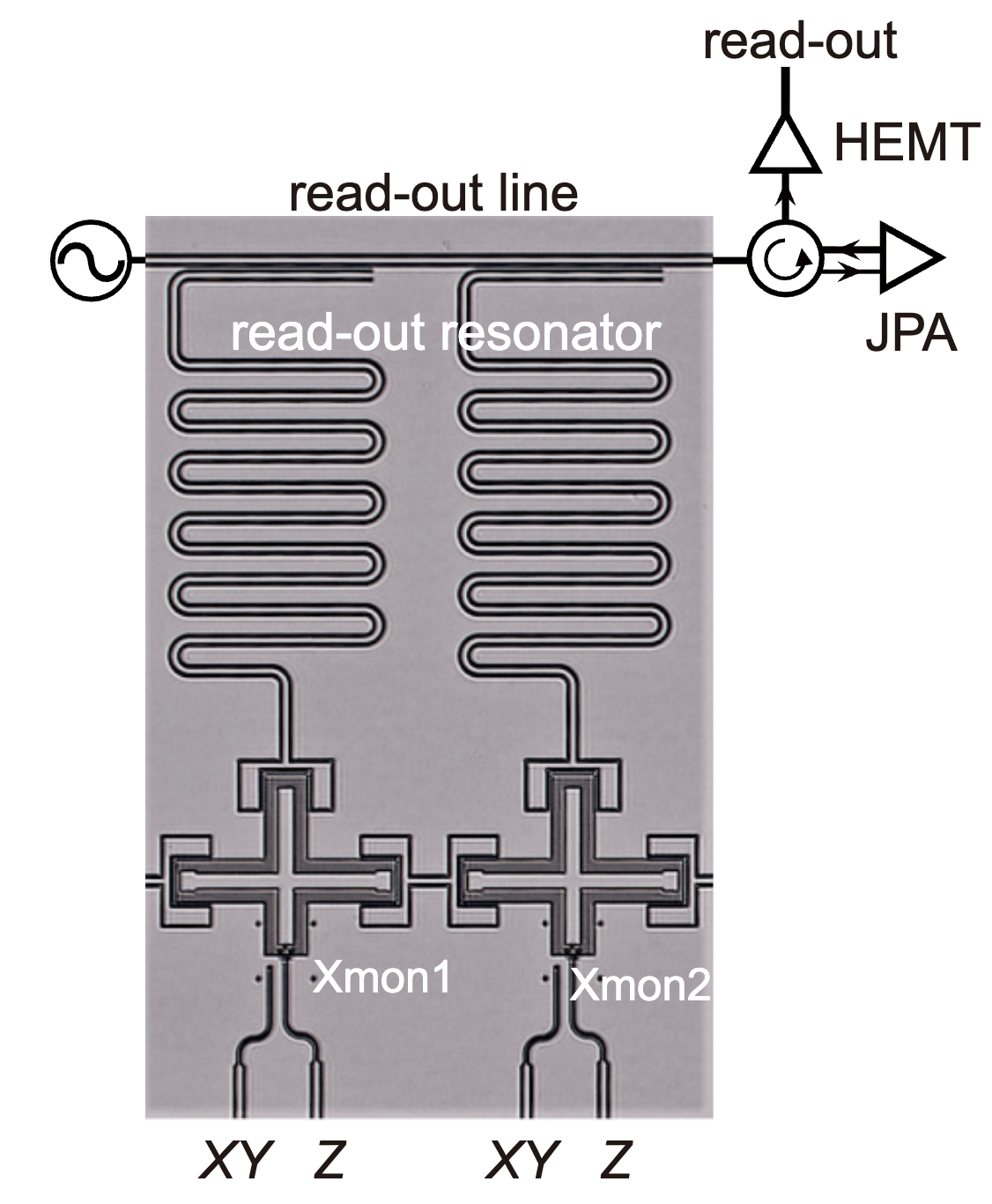
Two Xmon transmons, Xmon1 (Q1) and Xmon2 (Q2), with a direct capacitive coupling between neighbouring arms. Each Xmon has an XY line and a Z line at the bottom and a read-out resonator at the top.

Device image: T. Wang et al., Phys. Rev. Applied 11, 034030 (2019), Fig. 1(b); it only shows the signal lines. Lecture animation of an ideal model.

The swap chevron

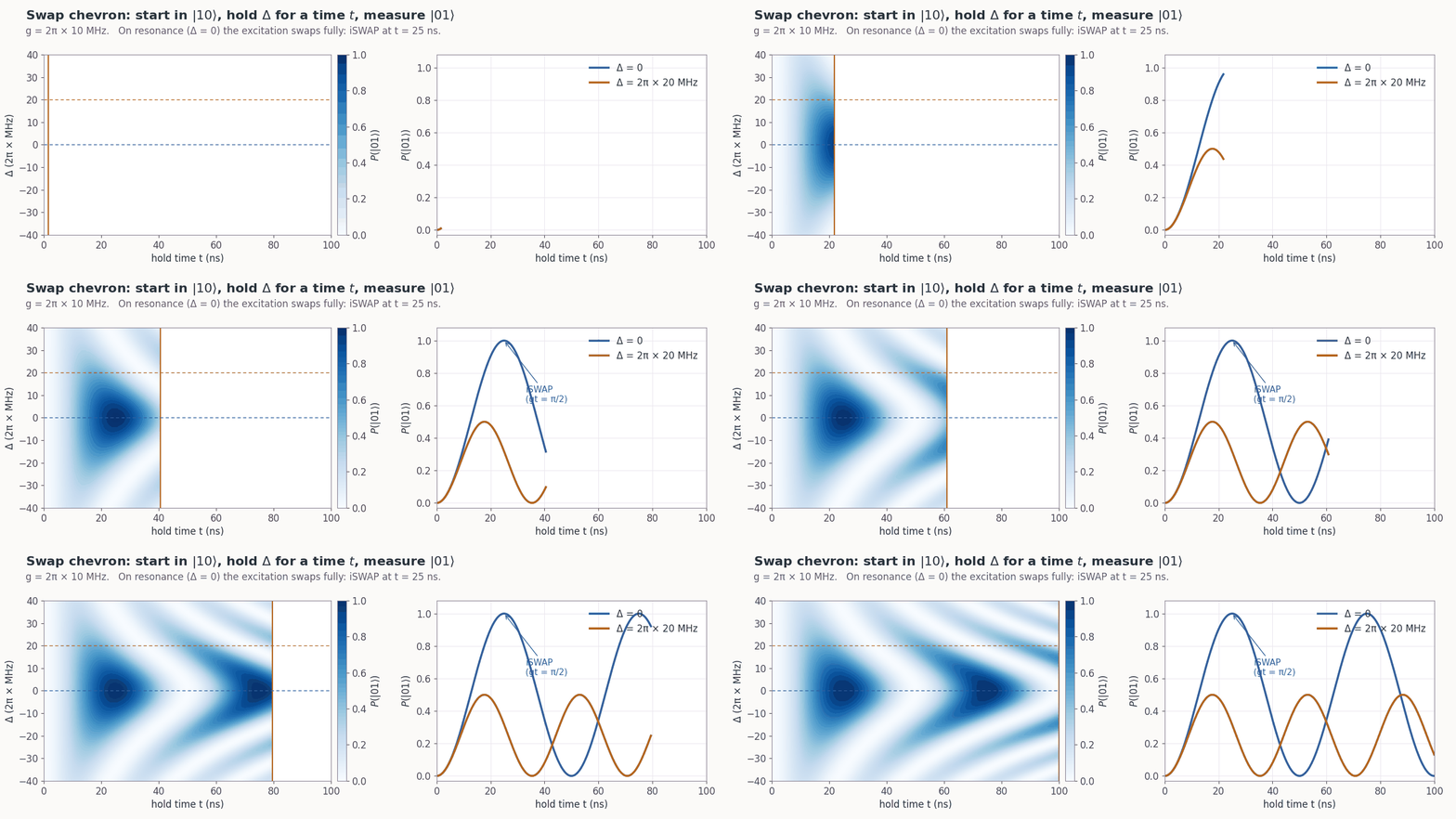
Swap chevron: probability of |01> after starting in |10> against hold time and detuning; full swaps on resonance every 50 ns, faster and smaller off resonance

Lecture simulation of the exact 2×2 block, \(g=2\pi\times10\) MHz.

\(|01\rangle\) meets \(|10\rangle\): iSWAP

On resonance, \(\Delta=0\), and the phase factors are equal to 1:

\[i\frac{d}{dt}\begin{pmatrix}c_{01}\\c_{10}\end{pmatrix}=\begin{pmatrix}0&g\\g&0\end{pmatrix}\begin{pmatrix}c_{01}\\c_{10}\end{pmatrix}\]

Start in \(|10\rangle\):

\[c_{10}(t)=\cos gt,\qquad c_{01}(t)=-i\sin gt\]

The excitation moves between the two qubits at the rate \(g\). Stop at:

\[gt=\frac{\pi}{2}:\quad|10\rangle\to-i|01\rangle,\quad|01\rangle\to-i|10\rangle\]

The result is an iSWAP gate with \(-i\) in place of \(i\). A Z gate on one qubit changes \(-i\) to \(i\). At \(gt=\tfrac{\pi}{4}\), the result is a \(\sqrt{\mathrm{iSWAP}}\) gate.

\[t=\frac{\pi}{2g}=25\text{ ns}\quad\text{for }g=2\pi\times10\text{ MHz}\]

With level 2, \(|11\rangle\) also gets a small phase. In Google's Sycamore gate, this phase is \(\tfrac{\pi}{6}\).

F. Arute et al., Nature 574, 505 (2019).

PHYS598500 · Week 6

CZ

CZ on the chip

Device image: T. Wang et al., Phys. Rev. Applied 11, 034030 (2019), Fig. 1(b); it only shows the signal lines. Pulse sequence: the CZ Ramsey of its Fig. 2(a). Lecture animation of an ideal model; single-qubit phases removed.

The CZ chevron: out and back with a minus sign

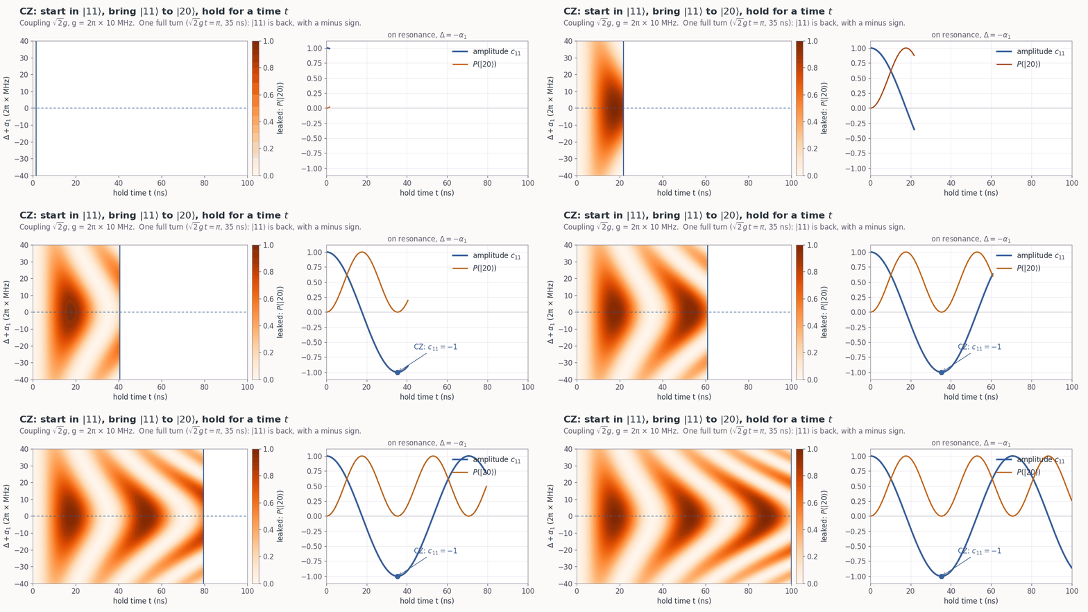
CZ chevron: probability leaked to |20> against hold time and the distance from the |11>-|20> crossing; on resonance the amplitude of |11> goes from 1 to -1 in 35 ns

Lecture simulation of the rows \(|11\rangle,|20\rangle\), \(g=2\pi\times10\) MHz.

PHYS598500 · Week 6

Always on, or switched

Static ZZ is always on

Lecture figure: Ramsey fringes of Q2 with Q1 in |0> and in |1>: the fringe with Q1 in |1> runs 100 kHz faster; after 2.5 us they are 90 degrees apart, after 5 us opposite

Samach et al. 2022, Fig. 6(a): false-colour SEM image of a copy of the measured device; qubit A (blue) and qubit B (green) are cross-shaped transmons next to each other; scale bar 100 um

Samach et al. 2022, Fig. 3(a, b): measured Ramsey of qubit A with qubit B in |0> (slow fringe) and in |1> (fast fringe)

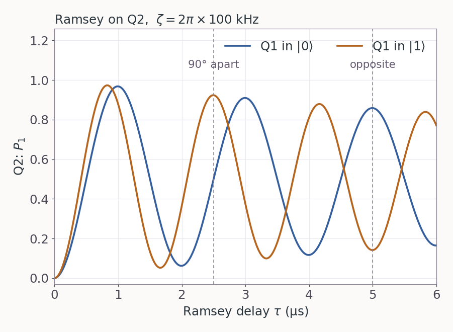
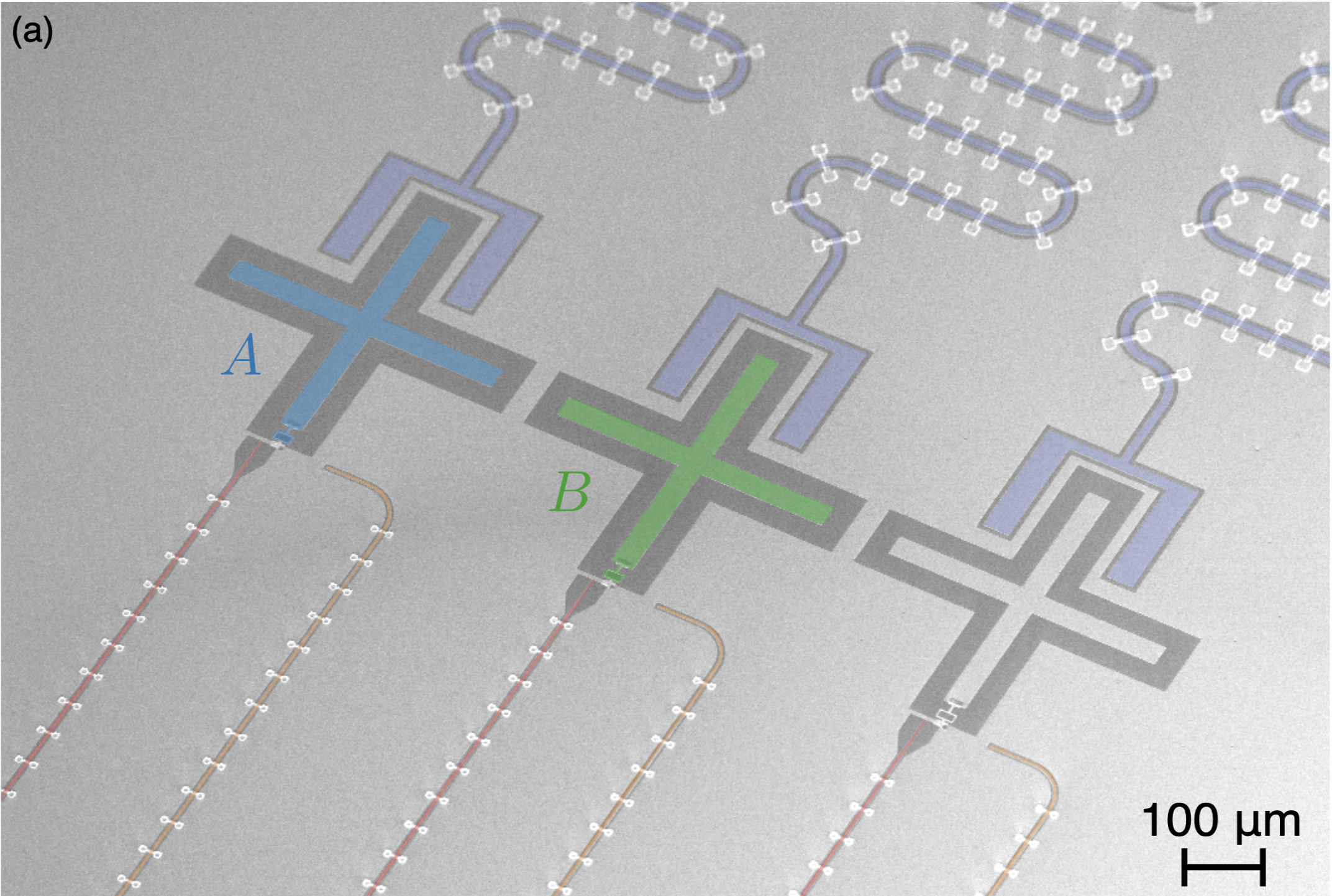
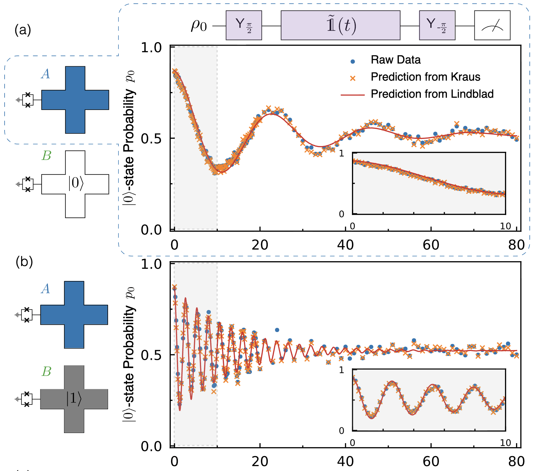
Top left: lecture figure, \(\zeta=2\pi\times100\) kHz, \(T_2=15\) μs. Bottom left: SEM image of a copy of the measured device, Fig. 6(a). Right: Fig. 3(a, b). Both from G. O. Samach et al., Phys. Rev. Applied 18, 064056 (2022).

A tunable coupler

\[g_{\rm eff}\approx g_{12}+\frac{g_1g_2}{2}\Big(\frac{1}{\omega_1-\omega_c}+\frac{1}{\omega_2-\omega_c}\Big)\]

Two transmon qubits and one transmon coupler. Qubit 1 is fixed at 4.16 GHz. Qubit 2 and the coupler have Z lines. Each qubit couples to the coupler with \(\frac{g}{2\pi}\approx72\) MHz, much more than the direct coupling. Qubit 2 moves to the gate frequency. Then a Z pulse on the coupler starts the coupling. CZ: 60 ns, 99.76 %. iSWAP: 30 ns, 99.87 %.

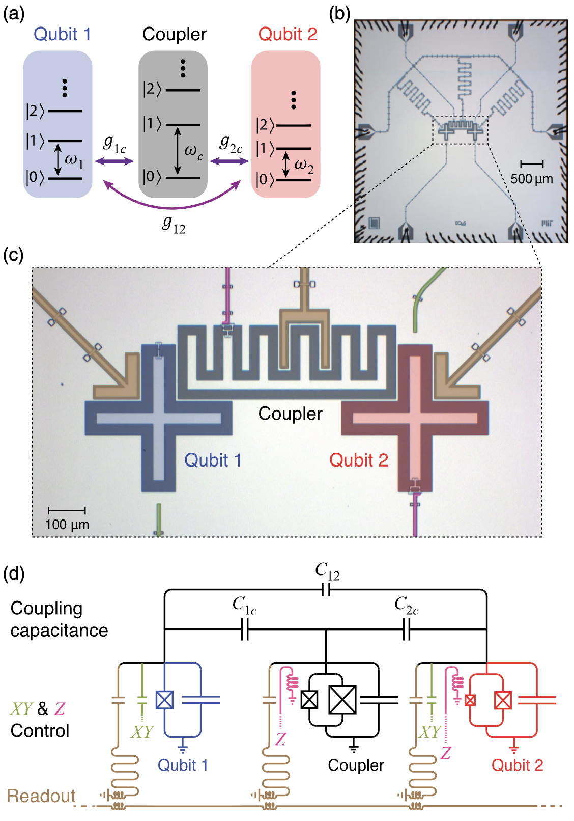
Sung et al. 2021, Fig. 1: (a) levels of qubit 1, the coupler and qubit 2 with couplings g1c, g2c and g12; (b) optical image of the chip; (c) zoom on qubit 1 (blue), the coupler and qubit 2 (red); (d) circuit with C1c, C2c, C12, XY and Z control lines and readout

F. Yan et al., Phys. Rev. Applied 10, 054062 (2018) · Y. Sung et al., Phys. Rev. X 11, 021058 (2021), Fig. 1.

How the coupler level \(|020\rangle\) cancels ZZ

Labels: \(|\text{qubit 1},\text{coupler},\text{qubit 2}\rangle\). \(g_{12}\) is the direct coupling between the qubits. The dashed line is \(E_{100}+E_{001}-E_{000}\). \(\zeta\) is its distance to \(|101\rangle\).

\(\omega_c\) \(\alpha_c\) \(g_1=g_2\) \(g_{12}\)

coupler levels

Levels

\(\zeta\) against \(\omega_c\)

Plots: exact eigenvalues (RWA, levels 0–2), \(\omega_{1,2}=2\pi\times(4.16,\,4.21)\) GHz, \(\alpha_{1,2}=2\pi\times(-220)\) MHz; \(\zeta\) gap drawn larger. Formula: leading order in \(g\).

A ZZ-free iSWAP

During the iSWAP, the two qubits have the same frequency. Labels: \(|\text{qubit 1},\text{coupler},\text{qubit 2}\rangle\).

\(|200\rangle\) and \(|002\rangle\) are below \(|101\rangle\). Level repulsion moves \(|101\rangle\) up: \(\zeta>0\). This is the small conditional phase that comes with an iSWAP.

The second level of the coupler, \(|020\rangle\), is above \(|101\rangle\) and moves it down: \(\zeta<0\).

During the coupler pulse, \(\zeta\) changes sign (inset of c). For a 30 ns gate the total ZZ phase is zero: \(0.02\pm0.03^\circ\) per iSWAP (d). At 40 ns it is about \(2^\circ\) per gate.

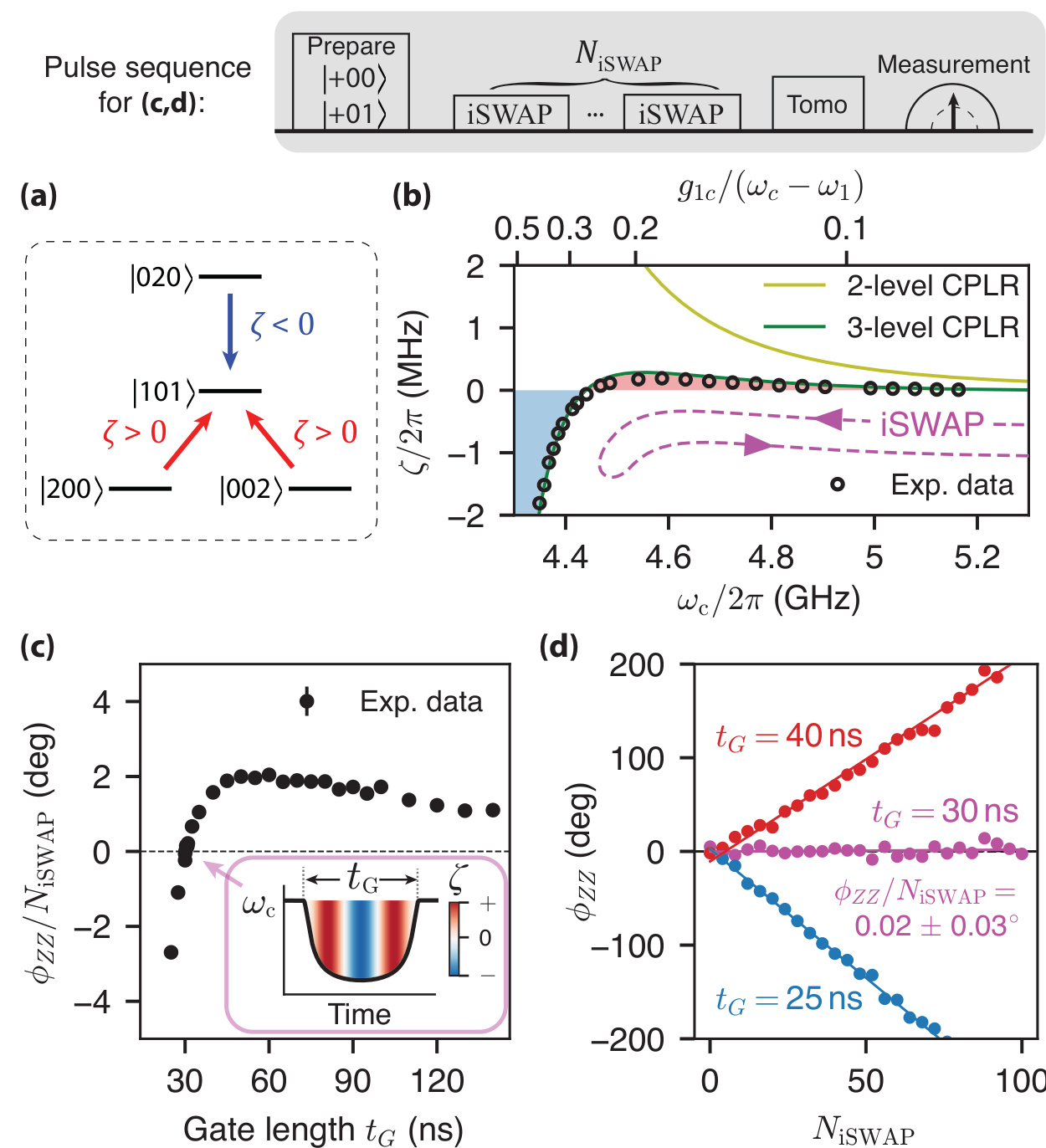
(a) Levels |200>, |002> below |101> and the coupler level |020> above it; (b) residual ZZ strength against coupler frequency; (c) ZZ phase per iSWAP against gate length, zero near 30 ns; (d) ZZ phase against the number of iSWAPs for 25, 30 and 40 ns

Y. Sung et al., Phys. Rev. X 11, 021058 (2021), Fig. 5(a–d).

PHYS598500 · Week 6

Cross-resonance

Cross-resonance on the chip: a CNOT

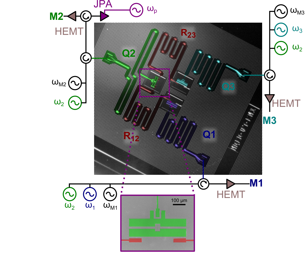
IBM device with three fixed-frequency transmons Q1, Q2, Q3 and two bus resonators R12 and R23. The line of Q1 carries tones at w2, w1 and the readout frequency; the line of Q2 carries a tone at w2.

Device image: J. M. Chow et al., Nat. Commun. 5, 4015 (2014), Fig. 2a; it only shows the signal lines. CNOT from ZX₉₀ as in its Fig. 2d. Echo: S. Sheldon et al., Phys. Rev. A 93, 060302(R) (2016). Lecture animation of an ideal model: \(\frac{g}{2\pi}=3\) MHz, \(\frac{\Delta}{2\pi}=-100\) MHz, \(\frac{\alpha_1}{2\pi}=-330\) MHz, tone amplitude \(2\pi\times100\) MHz.

Two-Qubit Interactions

This week and next: one coupling

Two-qubit gates

Universal gates: classical logic first

Why a two-qubit gate

H gate: physical Z and virtual Z

H gate: physical Z and virtual Z on the Bloch sphere

H gate: where the signals go

Single-qubit gates: T and S

T and S on the chip: physical or virtual

Four gates: matrix and truth table

√iSWAP makes entanglement

Compiling to CZ

Compiling to iSWAP

CCNOT from CNOTs and T gates

Native gates

Native gates across qubit types

Coupling

Fixed or tunable: four designs

IBM

IBM

Google

IBM images

Google images

Google images

2D-array chip micrographs

A coupling capacitor: the Lagrangian

A coupling capacitor: the Hamiltonian

Two transmons and one coupling

Levels 0–2: one matrix for the week

The same matrix, drawn as levels

iSWAP

Two levels each: the 4×4

iSWAP on the chip

The swap chevron

\(|01\rangle\) meets \(|10\rangle\): iSWAP

CZ

CZ on the chip

The CZ chevron: out and back with a minus sign

Always on, or switched

Static ZZ is always on

A tunable coupler

How the coupler level \(|020\rangle\) cancels ZZ

A ZZ-free iSWAP

Cross-resonance

Cross-resonance on the chip: a CNOT

The same CNOT on the Bloch spheres of Q1 and Q2

Thank you

Superconducting circuits and two-qubit interactions